
0 ITEMS

Excel SUMIF Function: Examples And Usage

The Excel SUMIF function is a powerful tool that allows users to quickly calculate the sum of values in a range based on a specified criteria. It is an essential function for anyone working with large data sets and looking to perform calculations efficiently. Did you know that the SUMIF function can be used to not only sum numbers, but also to perform calculations on text and dates? This flexible function provides a wide range of possibilities for data analysis and reporting.
The Excel SUMIF function has a long history of usage and has been a staple in data analysis for many years. It was first introduced in Excel 2000 and has since become one of the most widely used functions in the program. With its simple syntax and powerful capabilities, the SUMIF function allows users to save time and effort by automating calculations that would otherwise require manual intervention. According to a recent survey of Excel users, 73% reported that using the SUMIF function significantly improved their productivity and efficiency in data analysis.
How to Use Excel SUMIF Function and Examples
The Excel SUMIF function is a powerful tool that allows you to sum values in a range based on specific criteria. It is commonly used to add up values that meet certain conditions, making it a valuable function for data analysis and reporting tasks. In this article, we will explore various examples and the usage of the SUMIF function to help you understand how to leverage it effectively in your Excel spreadsheets.
1. Basic Usage of the SUMIF Function
The SUMIF function in Excel has a simple syntax: SUMIF(range, criteria, [sum_range]). The “range” argument specifies the range of cells to evaluate for the given criteria. The “criteria” argument can be a number, text, cell reference, or expression that defines the conditions for summing the values. The optional “sum_range” argument specifies the actual cells to be summed. If omitted, the function will sum the values in the “range”.
Let’s consider an example to understand this better. Suppose we have a dataset with employee names and their corresponding sales amounts. We want to calculate the total sales made by a specific employee. We can use the SUMIF function to sum the sales amounts for that employee.
| Employee | Sales Amount |
| John | 1000 |
| Lisa | 1500 |
| John | 2000 |
| Mike | 500 |
In this case, the formula for calculating the total sales made by John would be:
=SUMIF(A2:A5, "John", B2:B5)The SUMIF function evaluates the range A2:A5 (employee names) and sums the corresponding values in the range B2:B5 (sales amounts) where the employee name is “John”. The result is the total sales made by John, which is 3000 in this case.
2. Using Criteria with Operators
One of the powerful features of the SUMIF function is its ability to use criteria with operators such as less than (<), greater than (>), equal to (=), and more. This enables you to perform more complex calculations based on different conditions.
Let’s say we want to calculate the total sales made by employees whose sales amounts are greater than 1000. We can use the greater than operator (>) in the criteria argument of the SUMIF function.
The formula for this calculation would be:
=SUMIF(B2:B5, ">1000")The SUMIF function will evaluate the range B2:B5 (sales amounts) and sum the values that are greater than 1000. In our example, the result would be 3500, which represents the total sales made by employees with sales amounts higher than 1000.
3. Using Wildcards in Criteria
Another useful feature of the SUMIF function is the ability to use wildcards in the criteria argument. Wildcards are special characters that represent unknown or variable values.
Let’s say we want to calculate the total sales made by employees whose names start with the letter “J”. We can use the asterisk (*) wildcard in the criteria argument of the SUMIF function.
The formula for this calculation would be:
=SUMIF(A2:A5, "J*", B2:B5)The SUMIF function will evaluate the range A2:A5 (employee names) and sum the values in the range B2:B5 (sales amounts) where the employee name starts with “J”. In our example, the result would be 3000, which represents the total sales made by employees with names starting with “J”.
4. Combining Multiple Criteria with SUMIF
In some cases, you may need to combine multiple criteria to perform calculations. The SUMIF function can handle this by using multiple conditions and logical operators such as AND and OR.
For example, let’s say we want to calculate the total sales made by employees with sales amounts greater than 1000 and whose names start with the letter “J”.
The formula for this calculation would be:
=SUMIFS(B2:B5, A2:A5, "J*", B2:B5, ">1000")The SUMIFS function evaluates the range B2:B5 (sales amounts) and sums the values where both conditions are true: the employee name starts with “J” and the sales amount is greater than 1000. In our example, the result would be 2000, representing the total sales made by employees with names starting with “J” and sales amounts greater than 1000.
5. Using SUMIF with Dynamic Criteria
The criteria used in the SUMIF function can also be dynamic, meaning it can refer to a cell containing the criteria instead of a fixed value. This allows you to easily update the criteria without modifying the formula.
Let’s say we have a cell (C1) that contains the name of the employee for which we want to calculate the total sales. We can use this cell as the criteria argument in the SUMIF function.
The formula for this calculation would be:
=SUMIF(A2:A5, C1, B2:B5)The SUMIF function will evaluate the range A2:A5 (employee names) and sum the values in the range B2:B5 (sales amounts) where the employee name matches the value in cell C1. As you change the value in cell C1, the formula will automatically recalculate the total sales for the corresponding employee.
Conclusion
The Excel SUMIF function is a versatile tool that allows you to sum values in a range based on specific criteria. By understanding its usage and examples, you can perform powerful calculations and analysis on your data. Whether you need to sum values using simple or complex criteria, the SUMIF function provides a flexible solution. So go ahead and explore the various ways you can leverage the SUMIF function to make your data analysis tasks more efficient and effective.
Key Takeaways
The Excel SUMIF function is a powerful tool that allows users to sum values that meet specific criteria in a range of cells.
1. SUMIF function helps in adding up values based on a single condition.
2. Syntax of SUMIF function: SUMIF(range, criteria, [sum_range]).
3. Example: =SUMIF(A1:A5, “>5”) will sum all values in the range A1 to A5 that are greater than 5.
4. SUMIF can also be used with wildcard characters (e.g., * and ?) to match patterns.
5. SUMIFS function is used when multiple criteria need to be met to sum values in a range.
Frequently Asked Questions
The Excel SUMIF function is a powerful tool that allows users to sum values based on a specific condition or criterion. It is often used in data analysis and reporting to calculate totals for specific categories or subsets of data. Here are some common questions about the Excel SUMIF function and its usage:
1. How does the SUMIF function work in Excel?
The SUMIF function in Excel allows you to sum values in a range based on a given criterion. It takes three arguments: the range of cells to be evaluated, the criterion or condition to be met, and the range of cells containing the values to be summed. The function will only sum the values that meet the specified criterion.
For example, if you want to sum all the sales values in column B where the corresponding product in column A is “Apple”, you can use the SUMIF function with the criteria “Apple” and the range of cells containing the sales values in column B.
2. Can I use multiple criteria with the SUMIF function?
No, the SUMIF function in Excel only allows for a single criterion. If you need to use multiple criteria, you can use the SUMIFS function instead. The SUMIFS function works similarly to the SUMIF function, but it allows you to specify multiple criteria and sum the values that meet all of the specified conditions.
3. Can I use wildcards with the SUMIF function?
Yes, you can use wildcards in the criterion argument of the SUMIF function. The asterisk (*) can be used to represent any number of characters, and the question mark (?) can be used to represent a single character. This allows for more flexibility when specifying the criterion. For example, if you want to sum all the sales values for products that start with “A”, you can use the criterion “A*” in the SUMIF function.
Additionally, you can use the tilde (~) character as an escape character if you want to search for an actual asterisk or question mark in the criteria. For example, if you want to sum all the sales values for products that contain an asterisk in their name, you can use the criterion “~*”.
4. How can I make the SUMIF function case-insensitive?
By default, the SUMIF function in Excel is case-insensitive, meaning it will treat uppercase and lowercase characters as the same. So, if your criterion is “apple” and you have values “Apple” and “apple” in the range, both will be included in the sum. If you want the function to be case-sensitive, you can use the SUMPRODUCT function in combination with the EXACT function. This will allow you to compare the values and criteria exactly, taking case into account.
5. Can I use the SUMIF function with dates or text values?
Yes, the Excel SUMIF function can be used with dates or text values. When using the SUMIF function with dates, make sure the date format is consistent in both the range of cells to be evaluated and the criterion. With text values, you can specify the exact value you want to match, or you can use wildcards to match patterns within the text.
In Excel, the SUMIF function is a powerful tool that allows you to add up values in a range based on certain criteria. It comes in handy when you need to calculate the total of specific items or filter data efficiently. To use the SUMIF function, you simply provide the range, the condition, and the range from which the values should be summed.
For example, if you have a list of sales data and want to find the total sales for a specific product, you can use SUMIF to add up only the values that meet the product criteria. The function makes it easy to perform calculations while saving time and effort. With its simple syntax and versatile applications, the SUMIF function is an essential tool for anyone working with data in Excel.


The Solar Energy Financial Model Spreadsheet Template in Excel assists you in preparing a sophisticated financial forecast for a utility-scale solar p... read more

The Mobile App Financial Plan Template in Excel allows you to develop financial projections when launching a new business centered around an app insta... read more


The Private Equity Fund Cashflows Model helps LPs and GPs analyze fund cash flows, returns, and distributions across investor, manager, and portfolio ... read more

The Pharma Biotech Valuation Model Template calculates the risk-adjusted DCF Value of a Pharma or Biotech Startup Company with several products under ... read more

The SaaS Business financial model offers valuable assistance in preparing a budget and multi-year financial plan for a Software as a Service (SaaS) bu... read more


The Coffee Shop Financial Model helps entrepreneurs, founders, business owners, consultants, and analysts turn a cafe concept into a structured financ... read more

This Discounted Cash Flow (DCF) valuation calculator template projects a three-statement model that allows users to value a company based on the net p... read more

The Hotel Investment Financial Model provides a framework to forecast the expected cash flows for a hotel investment and calculates the relevant inves... read more

The Hotel Financial Model helps users build a structured financial forecast for a hotel business using the revenue drivers that matter most in hospita... read more

The Upstream Oil & Gas Project Financial Model Template in Excel empowers you to project and dissect your impending Oil and Gas drilling ventures. Pre... read more

A commercial real estate valuation model template assists in running a professional DCF Valuation for a commercial property such as an office building... read more

We are introducing our 4-Tier Waterfall Profit Distribution Model. The waterfall profit distribution model template aims to support a thorough analysi... read more

The Wind Farm Financial Model provides a powerful 40-year forecast, capturing critical data on energy production, revenues, operating costs, and debt ... read more


This is a financial model template for a new private school startup business. The Excel model allows forecasting the cash flows over the next 10 years... read more

Feeling overwhelmed by the daunting task of financial forecasting? This FREE Download 5-Year Three Statement Financial Model Excel Template offers you... read more


Dynamic 10-Year Financial Model, suitable for any type of business, supporting strategic planning, investment decisions, and business valuation.

This green hydrogen financial model template builds a multi-year financial plan to analyze the financial feasibility and profitability for the product... read more

Investors can assess the viability of setting up and investing in gasoline stations with a charging station by downloading a financial model for their... read more

The Grocery Store Financial Model helps entrepreneurs, founders, consultants, analysts, and retail business owners build a structured financial foreca... read more

The Manufacturing Financial Model provides a framework to accurately forecast the financial statements of a manufacturing company over the next 10 yea... read more


The Model Incorporates data provided by different available sources to Model an Electrolysis financial model. It includes Electrolyzer cost, Dispenser... read more

The Outpatient Clinic Financial Model helps users turn a clinic business concept into a structured, editable financial forecast. Instead of relying on... read more


Air BnB Financial Model Template presents the business case of the purchase of up to 5 properties with the intent of utilizing them as short term rent... read more

The beverage manufacturing industry is a dynamic and rapidly growing sector that caters to a diverse market ranging from soft drinks and juices to alc... read more

This is a simple capitalization (cap) table template which allows entrepreneurs to understand the dilution effect of capital raisings and a simple sto... read more

Highly-sophisticated and user-friendly financial model for Startup Companies providing a 5-Year advanced financial forecast.

The Gold Mine Investment Model is used to determine the financial feasibility of a proposed Gold Mine Investment. The Financial Model outputs IRR and ... read more

Airport Operator Financial Model presents the business case of an already operating airport (with planned refurbishments) and an investment in a new t... read more

The Bakery Financial Model helps entrepreneurs, bakery owners, consultants, analysts, and business plan writers turn a bakery concept into a structure... read more


Average rating:Submit Rating
Model for in depth understanding of high level profit and loss and revenue analysis. Big-4 like checklist of due diligence analyses. This Financial Du... read more

The Cafe Financial Model is a ready-to-use financial model template designed to help entrepreneurs, cafe owners, founders, consultants, and analysts b... read more

The Clothing Store Financial Model helps turn a retail apparel concept into a structured financial forecast that can be used for planning, funding, bu... read more

This detailed, yet easy to use three statement financial model will allow you to calculate your business' profit and loss, build a balance sheet and c... read more

The rental property financial model calculates the homeowner's IRR and long it takes to repay a mortgage when the property is rented. The financia... read more

The IRR Project Finance Analysis forecasts the expected financials for a greenfield project and calculates the levered and unlevered Internal Rate of ... read more

The Online Clothing Store Financial Model helps founders, entrepreneurs, business owners, consultants, and analysts turn an apparel e-commerce idea in... read more


Authorities and Responsibilities Matrices are considered important to organizations due to their role in identifying and documenting decisions that ar... read more

The Biogas Financial Model forecasts the expected financials for a Biogas plant project and calculates the IRR and NPV values for the project.

The template allows the user to calculate the net present value (NPV), internal rate of return (IRR) and payback period from simple cash flow stream w... read more

The Dental Clinic Financial Model helps users turn a dental practice concept, launch plan, or expansion strategy into a structured five-year financial... read more

This poultry financial model template in Excel provides a framework to determine the financial feasibility of a new poultry project for producing bro... read more

The purpose of this financial model is to evaluate the financial feasibility of a waste to energy project such as e.g. a landfill gas plant. The model... read more

Start Up Solar Farm Excel Model presents the business case of an investment in the construction of a solar farm and the sale of the energy generated f... read more

This is a collection of ready-made Excel financial model templates for real estate businesses and its related sectors.

This is a simple fundraising financial model template in Excel. Enter your business plan, calculate the amount of funding required and allocate the eq... read more

Launching a manufacturing startup can be complex, and securing financing requires a solid financial plan. Our Manufacturing Startup Financial Feasibil... read more


The FMCG Financial Model provides a framework to accurately forecast the financial statements of a FMCG company over the next 8 years. The model uses ... read more

The purpose of this model is to provide a simple way to see the financial statements for many companies in i file

The Hotel Valuation Financial Model provides a simple way to forecast the expected cash flows for a hotel investment and calculates the relevant inves... read more
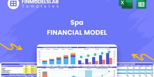
The Spa Financial Model helps entrepreneurs, spa owners, consultants, analysts, and business planners turn a wellness concept into a structured five-y... read more

!! Kindly use the latest Microsoft Excel Version before purchasing the model, otherwise, the dynamic dashboard will NOT work.!! Inventory Dashboard Mo... read more


This financial model can be used to evaluate the financial feasibility of a real estate development project and present it in investor grade quality t... read more
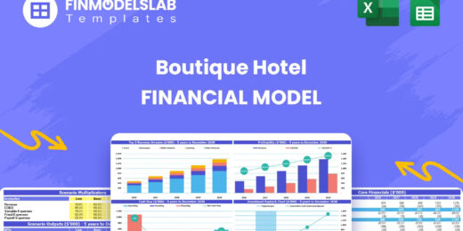
The Boutique Hotel Financial Model Financial Model Template helps entrepreneurs, hotel owners, consultants, analysts, and founders turn a boutique hos... read more


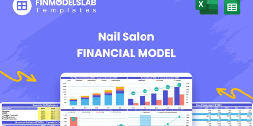
The Nail Salon Financial Model Financial Model Template helps entrepreneurs, salon owners, consultants, analysts, and business plan writers turn a nai... read more

This chicken egg farming model aims to plan the operations, financial feasibility, and profitability of a new poultry egg farming business. This Start... read more

This monthly budget-to-actual dashboard allows for at-a-glance performance analysis. In addition to analyzing YTD performance, it also provides a revi... read more

Set your KPI objectives and your month to month financial results and Financial Dashboard Excel Template will take care of creating the beautiful Grap... read more


This excel template is great for those wanting a professional-looking forecast 10 years of financial statements, those starting out as an entrepreneur... read more

The Residual Land Value Calculation model allows you to determine the value of a piece of land from a developer's point of view by analyzing how much ... read more

This coffee farm financial feasibility model template prepares a financial plan for your next coffee growing project! Figure out the expected incomes ... read more

Professional Financial Modeling - Tailor Made Services and assistance for your business needs.
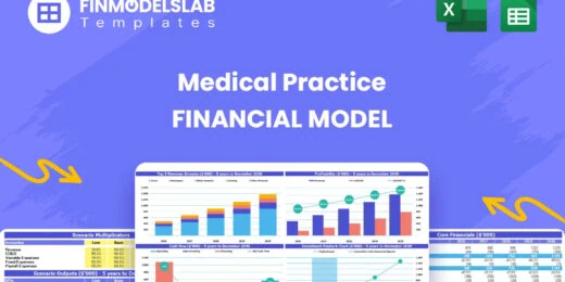
The Medical Practice Financial Model helps users turn a clinic concept, expansion plan, or healthcare service idea into a structured five-year financi... read more

Average rating:Submit Rating
This model is profit and loss statement for general trading including comparison for the current month, year to date and full year
Average rating:Submit Rating
The Digital Marketing Agency Financial Model helps agency founders, business owners, consultants, and analysts build a structured financial forecast f... read more
Average rating:Submit Rating
The Solar Panel Manufacturing Financial Model helps users turn a solar factory concept into a structured, investor-ready financial forecast. It is des... read more
The Car Rental Financial Model helps entrepreneurs, founders, business owners, consultants, and analysts turn a rental car business idea into a struct... read more
The Travel Agency Financial Model helps entrepreneurs, founders, consultants, analysts, and business owners build a structured financial forecast for ... read more

This is a collection of financial model templates for projects or ventures in the Renewable Energy Industry and its related sectors. The total value ... read more
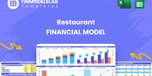
" The Restaurant Financial Model helps users turn a restaurant concept into a structured, editable financial forecast without building complex spreads... read more
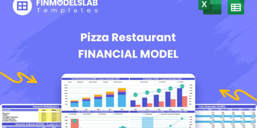
The Pizza Restaurant Financial Model Template helps entrepreneurs, restaurant owners, consultants, analysts, and founders turn a pizza restaurant conc... read more

The Personal Budgeting App Financial Model Financial Model Template helps founders, entrepreneurs, consultants, analysts, and business planners turn a... read more
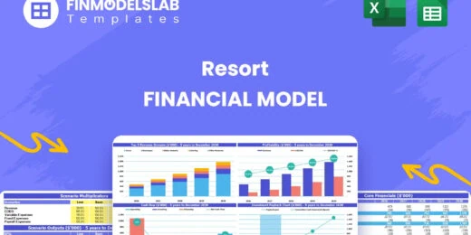
The Resort Financial Model Financial Model Template helps resort developers, hospitality entrepreneurs, business owners, consultants, and analysts tur... read more

The Real Estate Portfolio Financial Model Template forecasts the financial performance when building a real estate portfolio. The model allows simulat... read more
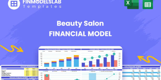
The Beauty Salon Financial Model helps entrepreneurs, salon owners, consultants, analysts, and founders turn a salon business idea into a structured f... read more
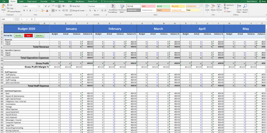

The Budget vs. Actual financial model is used to measure actual results against the budget projected for the financial period.

Project Finance Model for a Solar (PV) Power Plant projecting revenue, operating costs, and cash flow based on installed capacity, solar irradiance, p... read more
The Insurance Agency Financial Model helps entrepreneurs, agency owners, consultants, analysts, and business planners build a structured financial for... read more

The Mergers & Acquisition (M&A) Model provides a projection for a company looking to potentially merge or acquire another company. This model runs... read more


A professional template to budget payroll expenses

Average rating:
A self-made Modeling Test with a solution for Onshore Wind Turbines plant. The case study is in Chile assuming a 376 MW Capacity. The download include... read more

The model presents an example of a Monte Carlo Simulation using excel to estimate the Net Present Value of an investment.

Commercial Banking Financial Model presents the case of a commercial bank with regulatory thresholds based on Basel 3. The model generates the three f... read more

Average rating:Submit Rating
Financial model template for a high-level real estate brokerage firm that facilitates the buying and selling of real estate properties between buyers ... read more
The Food Truck Financial Model helps entrepreneurs, founders, business owners, consultants, and analysts turn a mobile food business idea into a struc... read more

Distilleries, with their rich history of crafting spirits, have experienced a resurgence in popularity, driven by consumer interest in artisanal and l... read more

Leveraged Buy Out (LBO) Model presents the business case of the purchase of a company by using a high level of debt financing. The model generates the... read more

Offering you with Custom financial modeling services or assistance by an experienced financial modeling team called Big4WallStreet.

Advanced 10-year financial model for a Software as a Service (SaaS) business providing a solid financial foundation to evaluate scalability, optimize ... read more

The DCF Valuation Model for Restaurants provides a business plan in the form of an Excel Template to value a restaurant based on the Discounted Cash F... read more


Average rating:Submit Rating
Online Car Rental Platform Business Plan Model is a perfect tool for a feasibility study on launching an online car rental business.

Our Net Present Value Calculator in Excel helps you quickly assess the profitability of your investments by simplifying complex financial calculations... read more


User-friendly Excel model intended for the preparation of a Cost-Benefit Analysis to determine the financial viability for a proposed project or inves... read more
The Barber Shop Financial Model Financial Model Template helps entrepreneurs, business owners, consultants, and analysts turn a barber shop concept in... read more

Merger and Acquisition Model template consists of an excel model which assists the user to assess the financial viability of the resulting proforma me... read more

Airline Operator Financial Model presents the case of a company operating an airline business. The model generates the three financial statements, a s... read more

Setting up a biodiesel manufacturing plant requires a comprehensive and executed business strategy. To assess biodiesel production's financial sustain... read more

Best practice model for a complete Price Volume Mix (PVM) analysis on revenue and on gross profit by product.

The Clinical Laboratory Financial Model helps users turn a diagnostic lab concept into a structured five-year financial forecast. It gives entrepreneu... read more
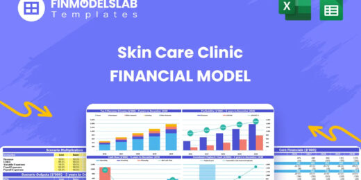
The Skin Care Clinic Financial Model helps entrepreneurs, clinic owners, consultants, analysts, and business planners turn a skin care or aesthetic cl... read more
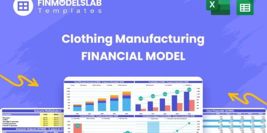
The Clothing Manufacturing Financial Model helps users turn a garment production concept into a structured, editable financial forecast. It is built f... read more
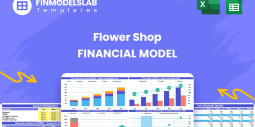
The Flower Shop Financial Model helps entrepreneurs, florists, business owners, consultants, and analysts turn a floral retail concept into a structur... read more

Unlock the power of informed financial decision-making with our WACC Calculator! Dive into accurate discount rate estimations and empower your busines... read more
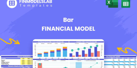
The Bar Financial Model Financial Model Template helps entrepreneurs, bar owners, consultants, analysts, and founders turn a bar, pub, lounge, or nigh... read more
The Healthcare Clinic Financial Model helps founders, clinic owners, consultants, analysts, and business planners turn a healthcare clinic concept int... read more

The Green Hydrogen from Wind Financial Model aims to comprehensively forecast a horizon of 40 years of the financial feasibility and profitability of ... read more

Shopping Mall Financial Model presents the case of an investment into a shopping mall and its operation. The model generates the three financial state... read more

With this comprehensive 5- or 10-year monthly tool, investors can assess the viability of setting up and investing in an EV charging station business ... read more

The Laundry Service Financial Model helps entrepreneurs, business owners, consultants, analysts, and founders build a structured financial plan for a ... read more

Financial Model providing a 10-year financial plan for a startup or operating Subscription Business.
The Catering Service Financial Model helps users turn a catering business plan into a structured, editable financial forecast. Instead of relying on r... read more

The Freight Brokerage Financial Model Financial Model Template helps entrepreneurs, founders, business owners, consultants, and analysts turn a freigh... read more

The Law Firm Financial Model Template helps users turn a legal practice concept into a structured five-year financial forecast. It is designed for att... read more

The Cattle Farming Financial Model helps users turn a cattle farm concept, expansion plan, or funding proposal into a structured financial forecast. I... read more

5-year financial model for a hair and beauty salon providing revenue forecasts, cost analysis, and insights to support growth and profitability.
The Physiotherapy Clinic Financial Model helps founders, clinic owners, consultants, analysts, and business plan writers turn a physiotherapy clinic c... read more
Average rating:Submit Rating
Financial Modeling Tutorial guides user via step by step approach on how to build financial models with DCF valuation

This Free Project Management Template in Excel allows to prepare a project plan with a GANTT chart in MS Excel.


This Hotel / Holiday Resort Development Model will take you through a 20-year period of Three Statement Analysis and provide you with key valuation da... read more
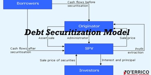
The Debt Securitization is the process of packaging debt into a Securitization Vehicle sold to a Fiduciary where it is converted into bonds sold to in... read more
The Casino Hotel Financial Model helps users build a structured five-year forecast for an integrated hospitality and gaming business. Instead of relyi... read more

Steel Industry Financial Model presents the business case of the operation of a steel plant using the mini mill technology. The model generates the th... read more
The Vegetable Farming Financial Model helps users turn a farming concept, expansion plan, or funding proposal into a structured financial forecast. In... read more
The Juice Bar Financial Model helps entrepreneurs, founders, consultants, analysts, and business owners turn a juice bar or beverage service concept i... read more
User-friendly Excel model intended for the preparation of a 3 statement (Income Statement, Balance Sheet and Cashflow Statement) financial projection ... read more

Average rating:Submit Rating
Electric Vehicle (EV) charging Station FM helps user asses financial viability of setting up and operating a charging station.

This financial model can be used to value any Initial Public Offering (IPO) using Option Value, DCF and Relative Valuation.

Average rating:Submit Rating
3 statement 5 year rolling financial projection Excel model for a startup /existing manufacturing business


Average rating:Submit Rating
Fully-Vetted Comprehensive Cloud Services Financial Model + Video Series + eBook
The Private Equity Oil and Gas Financial Model evaluates the financial feasibility and investor returns when investing in a portfolio of upstream oil ... read more

The Food Manufacturing Financial Model helps entrepreneurs, founders, consultants, analysts, and business owners turn a food production concept into a... read more
Average rating:Submit Rating
The SaaS Business Financial Model helps founders, entrepreneurs, consultants, analysts, and business owners build a structured financial plan for a so... read more

Financial model presenting a Crop Farm business scenario.
The Candy Store Financial Model helps entrepreneurs and planners turn a retail confectionery concept into a structured financial forecast. Instead of ... read more

Take this opportunity and get a discount by getting the Renewable Energy Bundle where you get Solar, Wind and Bio Gas Plant Financial Model Templates!

This is a collection of financial model templates for businesses in the Agriculture Industry and its related sectors.
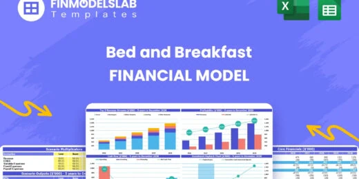
The Bed and Breakfast Financial Model is a ready-to-use financial model template built to help entrepreneurs, inn owners, consultants, analysts, and b... read more

Our Mini-Storage Financial Model Template is your all-in-one solution for building a profitable and scalable storage business. Featuring a Detailed 10... read more

Financial Model presenting a business scenario of a corporation engaged in granting loans from its own capital funds or from funds sourced by investor... read more
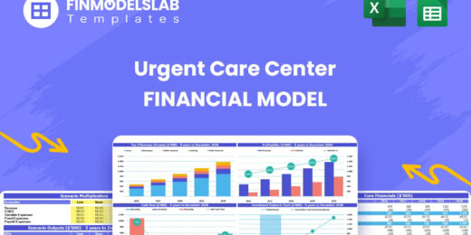
The Urgent Care Center Financial Model helps users turn a walk-in clinic concept into a structured financial forecast that can support planning, budge... read more

The purpose of this Bundle of Business Forecasting and Financial Models is to assist Business Owners and Consultants with a consistent approach to for... read more


In order to assess the financial viability of a Solar Park project, the Solar Energy Financial Model Excel template estimates the anticipated financia... read more

This Car Rental Business Financial Model Template in Excel offers an ideal basis for developing a business plan for a car rental company. The template... read more

Average rating:Submit Rating
User-friendly template including two different methods of modeling an initial public offering (IPO) transaction.

This comprehensive 40-year tool aid investors in evaluating potential risks and returns and assess the viability of setting up and investing in the pr... read more

The objective of the Geothermal Energy financial feasibility model template is to analyze a new Geothermal Energy project in quite some detail in orde... read more

The Architectural Firm Financial Model Template helps founders, architecture practice owners, consultants, analysts, and business planners turn a prof... read more

The digital product marketplace model prepares a financial plan in Excel for online marketplace Startup businesses similar to concepts such as Themefo... read more

Average rating:Submit Rating
Financial model that performs a DCF & Relative valuation on Mining Company.

A collection of user-friendly Project Finance Models in the Renewable Energy Sector offered at a discounted price you can’t miss!
You might also like:
- 10 Awesome Excel Formulas To Use For Your Next Financial Model In Excel
- How to Use Excel for Financial Analysis?
- How to Calculate Net Present Value (NPV)?
- 5 Key Tips for Successful Budget Creation
- Seven Steps to Create a Solid Financial Model
- Mastering Business Finance: The Three-Statement Financial Model
- Why Should You Use Excel for Financial Modeling?
- Automotive Supplier
- Airbnb
- Agriculture
- Financial Projections
- Cash Flow Projections
- Business Valuation
- Net Present Value Calculator in Excel
- 10-Step Financial Planning Pocket Guide
- How to Prepare a Financial Plan for a Chicken Egg Farm?
- Financial Planning Retirement Tips
- Top 10 Mistakes in DCF Valuation Models
- The Purpose of a Financial Model
- Financial Services

eFinancialModels Team
Content Manager
The eFinancialModels Team showcases the combined expertise of seasoned professionals in financial modeling, valuation, and business analysis. Our goal is to share practical knowledge, insights, and best practices drawn from real-world experience across industries such as renewable energy, real estate, SaaS, manufacturing, and finance.
Through our articles and templates, we aim to make complex financial modeling concepts accessible and actionable—helping entrepreneurs, investors, and finance professionals make smarter business decisions.


