A financial model in Excel is one of the most important tools used by Investment Bankers, Financial Modelers, and Analysts. Finance professionals spend a bulk of their work building assumptions and performing calculating valuations, assessing returns and risk, etc. in Excel. There are about 500+ formulas with 50+ financial formulas in Excel at a financial modeler’s disposal.

Regardless if it’s a basic or advanced Excel formula, every formula is useful. However, depending on the financial model in Excel you are building, you will not be using all of it. There will always be a select few as your go-to formulas.  In this article, we will go over advanced Excel formulas to help you build your next great financial model in Excel.

#1 Financial Formula In Excel: XNPV

The XNPV financial formula in Excel calculates the Net Present Value (NPV) of a project, asset, or investment based on the non-periodic cash flows generated and a discount rate. This advanced Excel formula is commonly used in financial models for capital budgeting and investment planning. Managers use the XNPV formula to gauge the profitability of a project, asset, or investment as well as comparing which one to undertake. If the result of the Excel XNPV formula is > 0, it means the project adds value to the firm, therefore, can be accepted.

The syntax for the Excel XNPV formula:

Where:

Rate                       The discount rate used over the length of the period (required argument)

Values                  Array or reference cells that represents the series of periodic or non-periodic cash flows (required argument)

                                Negative Values represent a cash outflow

                                Positive Values represent a cash inflow

Dates                    Series of date corresponding to the cash flows (required argument)

Example on how to use formula in Excel

Assume management decided to undertake a project to improve the marketing software for the Sales Team. Project X was started on the 1^st of June 2019 with an initial investment of $100,000. The discount rate is 10% (cell C2) and the series of cash flows (cells C6 to H6) generated from the project are non-periodic (cells C3 to H3). The Excel XNPV formula results in $13,149. Simply put, the cash generated from Project X is higher than the cost.

This advanced Excel formula is used in financial models in Excel for non-periodic cash flows.

#2 Financial Formula In Excel: XIRR

The XIRR financial formula in Excel calculates the Internal Rate of Return (IRR) for a non-periodic series of cash flows generated from a project, asset, or investment. This advanced Excel formula is used in financial modeling to analyze the potential rate of return and is compared to the company’s required rate of return. If the result of the XIRR financial formula in Excel is greater than the required rate of return, it means the project or investment adds value to the firm.

The syntax for the Excel XIRR formula

Where:

Values                  Array or reference cells that represents the series of periodic or non-periodic series of cash flows (required argument).

Dates                    Series of dates corresponding to the cash flows (required argument).

[Guess]                                Represents the approximation of the expected IRR (optional argument)

Example on how to use formula in Excel

Continuing with Project X’s example and using the Excel XIRR formula, Project X’s XIRR is 20%.

The XNPV and XIRR financial formulas in Excel are closely related to the NPV and IRR formulas in Excel. Learn more about the IRR vs NPV in the Context of Financial Decision-Making and use a free financial model in Excel template for IRR Project Finance Analysis

#3 Financial Formula In Excel: Excel PMT

The PMT financial formula in Excel is used to calculate the periodic total payment (principal and interest) of a loan, mortgage, or fixed-income investment. Hence, “PMT” stands for payment. This advanced Excel formula is commonly used in financial models dealing with debt schedules such as in commercial banking, real estate, etc.

The syntax for the Excel PMT formula is:

Where:

Rate                       The interest rate for the loan (required argument)

NPER                     The total number of periodic payments (required argument)

PV                          Present or the total value of the loan (required argument)

[FV]                       Future value or cash balance after last payment (optional argument)

[Type]                   Represents when payment is due (optional argument)

                                For end of the period payment: 0 or omitted

                                For beginning of the period payment: 1

Example on how to use formula in Excel

Assume in order to undertake Project X, management obtained a 5 year $100,000 bank loan with 5% annual interest to fund it.  Using the Excel PMT formula to determine the annual payments made at the end of the period, the result is $23,097.

#4 Advanced Excel Lookup Formula: INDEX MATCH

The INDEX MATCH advanced Excel formula is a combination of 2 separate formulas; INDEX and MATCH.

INDEX formula returns the value of a cell-based on the column and row number. Here is an article focusing on INDEX Function in Excel Explained & Examples

MATCH formula returns the position of a cell within a column or row. This formula is helpful for a financial model in Excel to Quickly Spot Data.

The combination is a good alternative to the more popular VLOOKUP formula. This combined formula is used in the financial model in Excel when looking up data from right to left in multiple columns and rows.

The syntax for the Excel INDEX formula

Where:

Array/ Reference             Represents the array or range of cells to get the value from (required argument)

Row_num                           Represents the row number (0, 1, 2, 3, etc.) of the Array or Reference argument (required argument)         

[Col_num]                          Represents the column number (0, 1, 2, 3, etc.)  of the Array argument (optional argument)

To understand in detail here an article focusing on INDEX Function in Excel Explained & Examples

The syntax for the Excel MATCH formula

Where:

Lookup_value                   Represents the value to find which can be numeric, text string, cell reference, or logical value (required argument)

Lookup_array                    Represents the range of cells to search from (required argument)

 [Match_type]                   Defines whether to return an exact match or the closest (approximate) match (optional argument)

Example on how to use formula in Excel

Using the Sales Team’s Employee List and Sales Data for 2019 and 2020 below, assume you want to perform a search for the Sales Agent Name and 2019 Sales per agent by simply inputting the Employee ID.

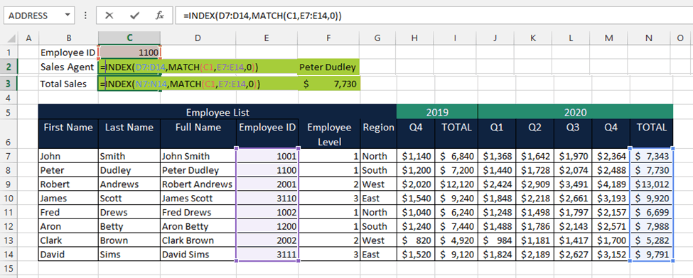
The INDEX MATCH formula makes the lookup process dynamic as it can search to the left of the table and allows flexibility in rows and columns.

#5 Handling Errors In Financial Models In Excel: IFERROR Formula

Errors found in a financial model in Excel compromises its integrity and the results it presents. The IFERROR formula is advanced Excel formula that checks for #N/A, #VALUE!, #REF!, #DIV/0!, #NUM!, #NAME?, and  #NULL errors within the financial model and returns an alternative value.

The syntax for the IFERROR formula:

Where:

Value                                    The value that needs to be tested or checked for error (required argument

Value_If_Error                  The value to return if an error is detected (required argument).

Example on how to use formula in Excel

Using the same Sales Team’s Employee List and Sales Data for 2019 and 2020 below, assume the user mistakenly inputs the wrong the Employee ID. When a Lookup formula does not find the value to search for, it results in the #N/A error.

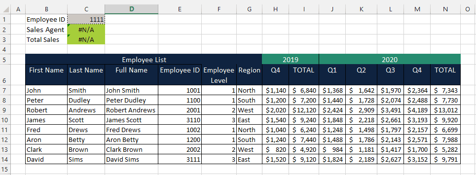
You can use the IFERROR formula to indicate instruct and inform the user to check and input the correct Employee ID by indicating “Employee Not Found” instead of just reflecting the error.

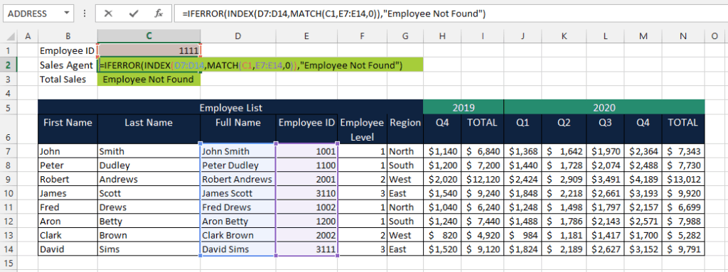
If you want to learn more about IFERROR advanced Excel formula, you may find these Answers to your Questions on IFERROR Function in Excel helpful.

#6 Data Cleaning For Financial Models In Excel: TRIM & PROPER

Financial model in Excel use data from different sources and applications, before financial modelers can use these for analysis it must be cleaned of unnecessary spaces and inconsistent text formats. Failing to do so will lead to errors in formula and results.

The TRIM formula is commonly used when the raw data contains leading and trailing spaces. Text data with unnecessary spaces affects the results of Lookup formulas (VLOOKUP, HLOOKUP, INDEX, MATC, etc.). Numerical values containing unnecessary spaces also affect Mathematical formulas (SUM, AVERAGE, etc.).

The syntax for the TRIM formula

Where:

Text                       The text string that contains spaces (requirement argument)

The PROPER formula is used to sets text in proper cases. For example, if the data for the financial model in Excel is composed of employee names, product names, descriptions, etc. and is presented in lowercase or upper case characters, the PROPER formula converts all the first character into uppercase and the remaining into lowercase.  

The syntax for the PROPER formula

Where:

TEXT                      The text string to be converted to (required argument0

Example on how to use formula in Excel

Continuing with the Sales Team’s Employee List and Sales Data for 2019 and 2020 below, assume the Full Names contain spaces with improper and inconsistent lower and upper case characters (Column D). With the TRIM PROPER formulas, you can remove any spaces and set proper case characters (Column E)

Use these Practical And Clear Techniques To Clean Data In Excel when building your next financial model in Excel.

#7 Advanced Excel Formula With Conditions: IF Statement Combined With Logical Operators

The Excel IF formula is a logical formula that checks whether a condition is met (TRUE) or not (FALSE). Combine this with other logical formulas such as AND, OR, Greater than ( > ), less than ( < ), etc. and a financial modeler has a powerful advanced Excel formula that can set multiple conditions and manipulate data to retrieve relevant information. These formulas are helpful in financial models in Excel for scenario and sensitivity analysis.

The syntax for the IF formula is

Where:

Logical_test                       Represents the condition to be tested as either True or False (required argument)

[Value_if_true]                Represents the value if the condition tested is met and therefore is True (optional argument)

[Value_if_false]              Represents the value if the condition tested is NOT met and is False (optional argument)

Delve deeper and Know What’s True Or False With IF Statement in Excel

Example on how to use formula in Excel

Using the Sales Team’s Employee List and Sales Data, you can perform an Annual Sales performance review for each sales agent using the Excel IF Formula. For example, you can base the 2 conditions to rate whether the sales agent reached the company target or not (below target).

Condition 1: 2020 Sales must be greater than ( > ) 2019 Sales AND

Condition 2: Q4 2020 Sales must be greater than ( > ) Q4 2019 Sales

#8 Advanced Excel Formula With Conditional SUM: SUMIF & SUMIFS

Excel’s conditional SUM formulas is one of the most important advanced Excel formulas used in a financial model in Excel. It combines a basic Excel formula, SUM, with an advanced Excel formula, IF Statement. The combination is designed to add values based on a set of conditions.

The SUMIF formula adds values based on a SINGLE condition. You can Analyze Financial Data with SUMIF Function In Excel

The SUMIFS formulas add values based on MULTIPLE conditions. You can Dissect Business Data with SUMIFS function in Excel

The syntax for the SUMIF formula:

Where:

Range                                   Specifies the range of cells to which the criteria must be applied (required argument)

Criteria                                 The single condition or criterion used to determine which cells will be added (optional argument)

Sum_range                         Range of cells with the numeric values that are to be added if the single condition or criterion is satisfied (optional argument)

The syntax for the SUMIFS formula:

Where:

Sum_range                                         Range of cells with the numeric values that are to be added if the conditions are met (required argument)

Criteria_range1                                The range of cells to be tested if (required argument)

Criteria1                                              The conditions which Criteria_range1 must be tested with (required argument)

[Criteria_range2, Criteria2,,,]     Additional ranges and criteria (optional argument)

Example on how to use formula in Excel

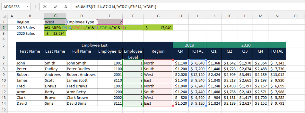
Continuing with the Sales Team’s Employee List and Sales Data, you can conditionally sum Sales by specifying the region using the SUMIF formula

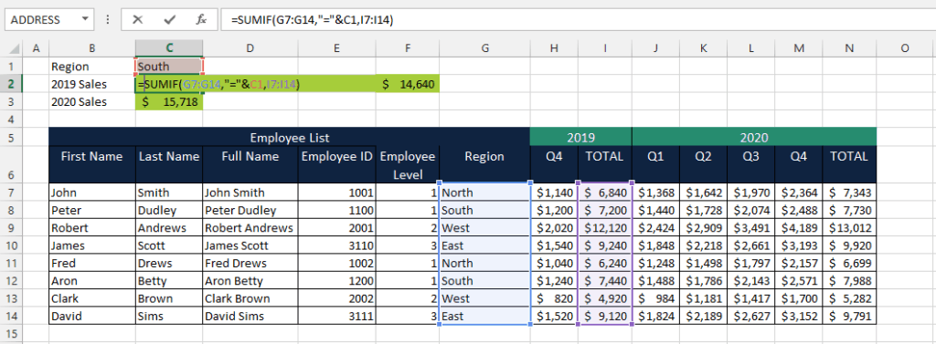
Or conditionally sum Sales per region and Employee ID using the SUMIFS formula.

#9 Excel CHOOSE Formula

The CHOOSE formula is not necessarily an advanced Excel formula nor can you consider it as a financial formula in Excel. This formula returns a value from a list of options based on a given position or index. But this is helpful in Excel financial models performing scenarios analysis. For example, by using the CHOOSE formula financial modelers and analysts can select and evaluate different scenarios (base, best, and worse case scenarios) that the Excel financial model can use to perform calculations.

The syntax for the CHOOSE formula

Where:

Index_Num                        Represents the position of the value to look up and must be a numerical value. This can be a formula of reference cell containing a numerical value (required argument)

Value1                                  The first value to choose from (required argument)

[Value2]                              The second value to choose from (optional argument)

Example on how to use formula in Excel

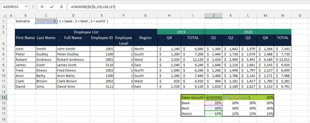
Assume the Sales Team’s Employee List and Sales Data for 2019 and 2020 below The Excel financial model below has 3 Sales Growth scenarios to select.

By simply entering #1,#2, or #3 scenario on cell C1, the Excel financial model uses the projected sales growth in its calculations.

#10 Excel’s & Operator

Data used for the financial model in Excel are not necessarily structured for financial analysis. Inputs from users and other sources as well as outputs from complex calculations must be combined to construct coherent financial information.  That’s why financial modelers need to combine or concatenate text and numbers from one or more cells.

Excel’s “&” (ampersand) operator is not entirely an advanced Excel formula as most financial modelers are familiar with the CONCATENATE formula to combine cells but it is a quicker and easier alternative is to use.

Example on how to use formula in Excel

Continuing with our example, to quickly combine the first name and last name to form the full name of each employee in the employee list, use the “&” operator to combine multiples cells.

Learn more on how to Combine Cells In Excel And Generate Dynamic Text With These 2 Formulas (Concatenate and “&” operator)

Advanced Excel Formulas And Financial Models In Excel

Finance professionals nowadays have a wide range of software and tools to use. But financial models in Excel has always been the preferred tool of choice for financial analysts and modelers. Without understanding how to use formulas in Excel, this will only be a data keeping tool or a high tech calculator.  Knowing advanced Excel formulas gives you enough room to build and design financial models to cater to every end-user’s needs. With financial formulas in Excel financial analysts and modelers can crunch data, analyze, and get answers to complex financial questions efficiently.