5 Steps to Create a Drop Down List Using Data Validation in Excel

A drop-down list, also called a data validation list in Microsoft Excel, is simply a list of choices to pick from- the list can be composed of any values such as numbers, dates, product codes, and specific texts like names, labels, etc. It’s called a drop-down list in Microsoft Excel because it remains hidden unless you decide to look into it and the menu of choices drops down for you.
Drop-down lists or data validation lists in Excel, are very useful for numerous reasons. The data validation list in Excel tells the user what input is required from them by simply choosing from the list which makes them input faster (takes out the guesswork) plus it prevents error messages; just to name a few.
Drop down or data validation lists in Excel are also used in building and analyzing financial models. A data validation list in Excel can be used to perform scenario and sensitivity analysis. A financial model with its numerous inputs, formulas, and links, is complex and the integrity of the model can be at risk due to human errors like misspelled words, invalid input, etc. By using data validation lists in Excel, the analyst can simply choose from the different standard inputs presented in the drop down list or even choose between base, best, or worst-case scenarios to create the results needed for decision making.
In this article, we will explain further what is data validation in Excel, how to create a drop-down in Excel, and how to use Excel data validation to update lists automatically, plus helpful tips.
How do I create a Drop Down List in Excel?
What is Data Validation in Excel
Data validation in Excel is a feature that controls what a user inputs into a cell and is found in the Data Tab of the ribbon.
It validates data input to make sure that these are accurate and consistent. For example, you can use data validation in Excel to make sure a number is between 1 to 5, a future date entry occurs in the next 90 days only, or a text description is no longer than 100 characters.
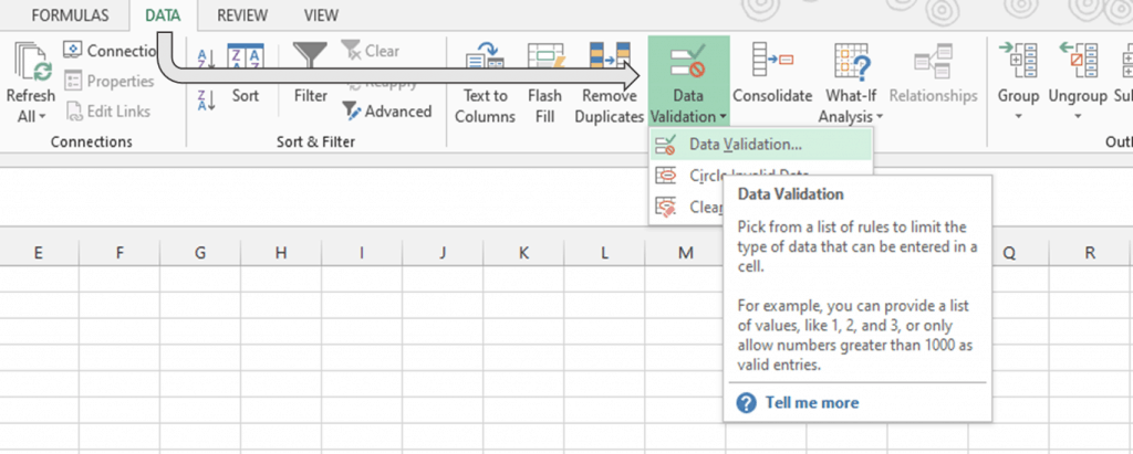
TIP: Use shortcut keys, press Alt + D + L.
Data validation in Excel is used to make drop down or data validation lists in Excel, its main purpose is to make a worksheet efficient. Excel’s data validation feature can detect any invalid data the user entered as well implement strict or lenient measures depending on validation rules you set.
Defining the Rules or Criteria of Data Validation in Excel
Upon accessing the Data Validation dialog box, you are presented with 3 tabs –Settings, Input Message, and Error Alert.
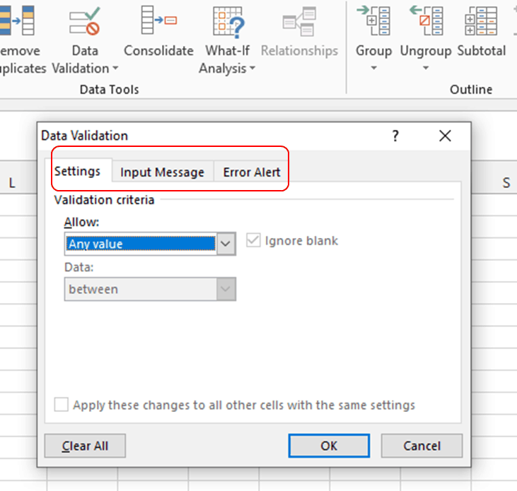
The Settings in Excel’s Data Validation
This is where the validation criteria are defined. There are 8 built-in rules including the ability to customize criteria and with each having its separate cell drop down options. Since this article is about the data validation list in Excel, we will focus on the “List” option from the menu.
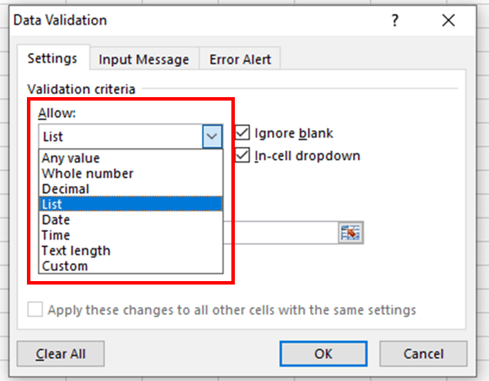
The Settings tab of the data validation in Excel includes 3 checkboxes.
- Ignore blank. Instructs Excel not to validate empty cells.
- In-Cell Dropdown. Allows drop down list in MS Excel to appear in the selected cell.
- Apply these changes to other cells with the same settings. Any changes made will also affect other cells in the same setting.
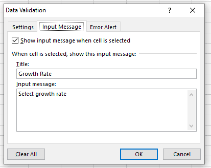
The Input Message in Excel’s Data Validation
If you prefer to display a message briefly explaining or instructing the user what to input in the cell, you can create this in the Input Message Tab. Take note this is optional and only based on your preference, you can opt not to show an input message and Excel’s data validation will not be affected by either choice.
The Error Alert in Excel’s Data Validation
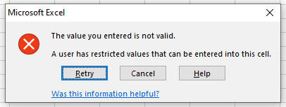
You can also display an error message alerting the user of an invalid data entered into the cell.
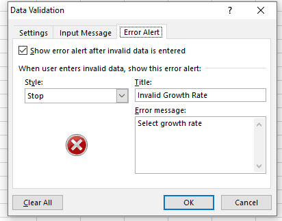
Excel’s data validation has 3 styles of error alert options:

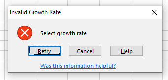
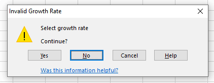
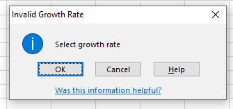
Similar to the Input Message, the Error Alert Message is also optional and purely based on your preference. Excel’s data validation will instead display a default Stop alert if you skipped this part.
How to (And Why) Create a Basic Drop Down or Data Validation List in Excel
Using a drop down list data validation or a drop down list in Excel is useful for the following reasons:
- Data validation lists in Excel tells users the required and expected input.
- Speeds up data input as options are already available and standardized.
- Improves data accuracy and limits, as well as prevents, errors depending on the error alert set.
- It helps make financial models and analysis more robust as it makes sure data is accurate and consistent.
- Data validation lists in Excel are flexible and dynamic. You can use the built-in rules or customize the criteria.
In Excel, there are two ways to create a drop down list:
- Use the Developer Tab OR
- Use Excel’s data validation feature
For this article, we will be discussing the latter. Let’s use the below example to illustrate.
Assume you are creating a revenue forecast model for a business.

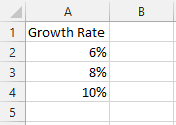
The model has 3 scenarios based on these forecasted revenue growth rates; 6%,8%, and 10%. To make the model efficient and limit errors, you want to create a drop down or data validation list in Excel. How to use Excel data validation to create this list?
Here are the steps to create a drop down list in MS Excel’s data validation:
Step 1 Create A Vertical List For The Data Validation In Excel
This is simply the directory or table detailing what the user sees and selects from when the drop down or data validation list in Excel appears. You can place the list on the same worksheet as your data validation list in Excel or separate worksheet. For this example, the list of the forecasted growth rates below was created in Sheet 2, cells A2 to A4.
Step 2 Select the Cell Where Data Validation List in Excel Appears
This is pretty simple and straightforward, you can position the drop down list in any cell on the worksheet. For the revenue forecast model, we select cell B1 in Sheet 1.

Step 3 Access Excel’s Data Validation Function
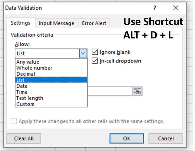
You can access Excel’s data validation under the Data Tab in the ribbon or the keyboard shortcut Alt + D + L (Other’s may use a different short cut, Alt + V + V + V but the result is the same).
Step 4 Fill the Required Fields under Settings and any Preferred Input or Error Alert Message
Since we are creating a data validation list in Excel, under “Allow” pick “List”.
Then reference the source list from where the users will pick from. For this data validation list in Excel example, the data source is located at Sheet 2 cells A2 to A4.
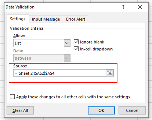
You can ignore the “Apply these changes to other cells with the same settings” tick box as we are only creating this data validation list in Excel.
Once done, you have the option to fill in the Input Message and Error Alert or skip these.
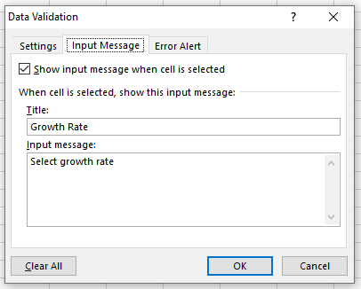
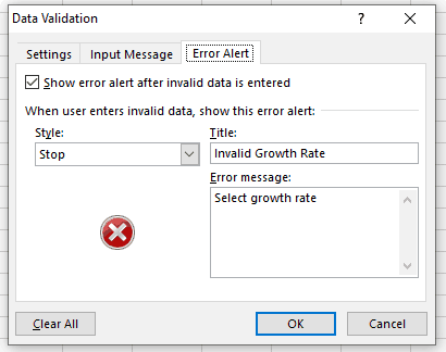
Step 5 Click OK and Test the Data Validation List in Excel
The Input Message appears once you clicked on the cell B1, the drop down or data validation list in Excel appears the choices to pick from.

The custom Error Alert appears when input is invalid.

Dynamic Data Validation List in Excel
Continuing with our example, assume you want to add new data to your source list – 4% revenue growth rate.
If you simply add 4% in Cell A5, this will not automatically update the data validation list in Excel nor include it as valid data input. How to use Excel’s data validation list in this instance?
One course of action is to insert a new row in between the cell ranges and input the 4% growth rate. This will update Excel’s data validation list as well as include it as valid data input.
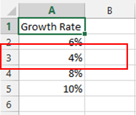
But this will be tedious and cumbersome, not to mention prone to errors especially if the source list is long and must be kept up to date. A second option is to use a dynamic data validation list in Excel.
A dynamic data validation list in Excel is composed of a source data that can be extended and therefore the data in the list can be added and removed.
Dynamic Data Validation List in Excel Using Excel Table and Named Range
To create a dynamic data validation list in Excel, first format the source list into an Excel table then create a named range. A named range, range name, or defined name is a descriptive name attached to a specific cell or range of cells that make it easier to use and identify data.
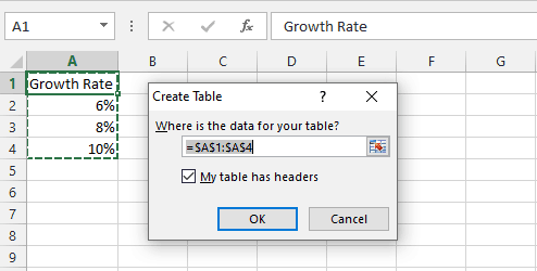
To format the source list into an Excel table, go to the Insert Tab then select Table. Or use the keyboard shortcut CTRL+T.
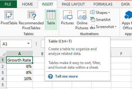
Always make sure to check the box for “My table has headers”.
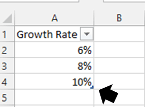
You have successfully converted the source list into an Excel table if you see this indicator at the last cell of your data list.
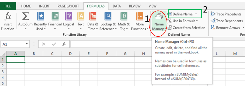
To create or define the named range, you can use either- Name Manager or Define Name functions found under the Formulas Tab.
To create the named range using Option 1-Name Manager, simply click New.
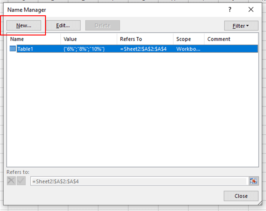
It is important to take note that under Name Manager, you can also view other tables and named ranges you created. The Table1 in the list represents the same table we just created.
Once you click New, a new dialogue box appears. This is the same dialog box that appears if you opted to create a named range using Option 2- Define Name.
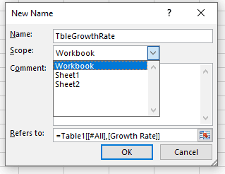
In the “Name” box enter one word (no spaces) name for the range, for this example, we will call the named range TbleGrowthRate.
Then identify the Scope of the name and, if you prefer, to input a comment or leave it blank.
Lastly and the most important part is the “Refers to” field. This directs Excel to the specific range of cells under the name “TbleGrowthRate”. Delete the pre-assigned name and click the ![]() icon.
icon.

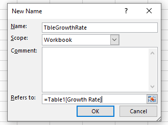
Reference the range of cells by clicking the top of the heading cell, this will automatically select the cells to be included. Take note not to reference the entire column.


Below is how the filled up dialogue box will appear, given you opt not to include any comment. Once done, click OK.
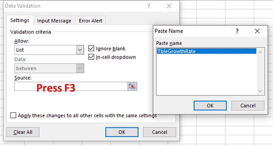
Next Step is to access Excel’s Data Validation function, choose “List” under Allow, and click on the Source box. Input the equal sign ( = ) and press F3 to select from the named ranges available. Look for your named range, “TbleGrowthRate”, and click OK.
Click OK again in the Excel’s Data Validation dialogue box.
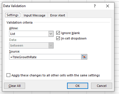
Recall, the Input Message and Error Alert messages are both optional.
At this stage, you have successfully created an Excel table and defined a named range. Now we can add the new 4% rate to our vertical list by simply entering it at the last cell in the table.
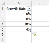
Doing so will now automatically update the drop down or data validation list in Excel.

Creating a Dependent Data Validation List in Excel Using Indirect Function
There are times where a single drop down or data validation list in Excel may seem to be too limited and you need to use two or more data validation lists in Excel such that the cell drop down options in the second drop down list is dependent on the selection made from the first drop down list.
Assume you want to further expand the revenue growth rates in your forecast model into two scenarios – Best and Worst:
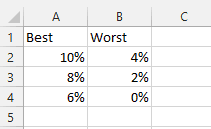
Essentially, there will be two data validation lists in Excel- the primary and the dependent lists.
- The primary data validation lists in Excel will be the two scenarios, Best and Worst
- The dependent data validation lists in Excel will be the respective growth rates of any of the two scenarios selected by the user.
How to use Excel’s data validation list in this instance?
Let’s start with the primary data validation list in Excel. Cell B2 is the chosen cell where the drop down list in MS Excel for the Scenario will appear.

Fill in the required fields in Excel’s Data Validation dialogue box.
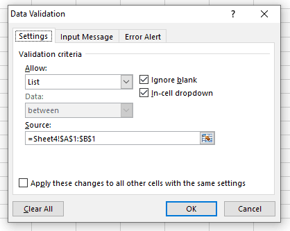
Take note the Source references the range A1 to B1 in the worksheet representing the 2 scenarios, Best and Worst.
Cell C2 is the chosen cell where the drop down list for the dependent list, Growth Rate, will appear.

To create the dependent data validation list in Excel, bear in mind this will be based on what the user selected from the primary list (Cell B2), we will use a custom formula called the INDIRECT function. This function returns a reference to a range and is useful as it will remain unchanged even if row or columns are inserted in the worksheet.
Similar to the primary list, fill the required fields in Excel’s Data Validation box. Under Source, we will use INDIRECT function and reference the selected option from our primary list- cell B2).
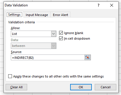
Once done, click OK.
The dependent data validation list In Excel is as follows:

The user will select one of the two Scenarios available from the data validation list in Excel in Cell B2.
Once selected, the user will then move on to selecting the growth rate from the data validation list in Excel (Cell C2) under the “Best” scenario.

Below presents the growth rate data validation list in Excel if the “Worst” scenario is selected instead.

Helpful Tips on How to Use Excel Data Validation List: How to edit Excel Drop Down List?
- There times where the Input Message box may block the cells underneath it (similar to below) especially if the message is a bit long. Use your mouse to move it anywhere on the activated worksheet.

- How to edit Excel drop down list? To edit (add or remove) the options from Excel’s data validation list, make the necessary changes in the Source box. Make sure to check the box for Apply these changes to all other cells with the same settings. Data validation in Excel will copy the changes made to all other cells with the same validation criteria.
- Validation Criteria created for a specific cell can also be used to validate other cells. Use CTRL+C to copy the cell’s validation criteria. Then select the other cells where the validation criteria will be applied, press CTRL+ALT+V to access paste special. From the menu, select Validation then click OK.
- To remove the drop down list created from data validation in Excel for a specific cell or range of cells, select the cells then click on the “Clear All” button on the bottom of the Excel’s data validation dialogue box. Make sure not to tick the checkbox for “Apply these changes to all other cells with the same settings”.
- On the other hand, to remove the drop down list in MS Excel data validation for ALL cells, select any cell with the drop down list. Then tick the checkbox for Apply these changes to all other cells with the same settings and click on the “Clear All” button on the bottom of the Excel’s data validation dialogue box.
Please check out this video about How to Create a Data Validation List in Excel:

