Roadmap To Understanding And Using SUMPRODUCT Function In Excel

The SUMPRODUCT function in Excel is one of the SUM Functions (SUM, SUMIF, SUMIFS) [link to pillar page] under the Math/Trigonometry Formulas. Using the SUMPRODUCT formula, it multiplies the range of cells or arrays then sums all the products.
If I ask you how often you use this function compared to other SUM functions and you answered rarely, I wouldn’t be surprised. It is sort of like the unpopular kid on the block or the quintessential last kid to get picked for a team. Almost everyone knows what it does but chooses not to use it. In financial modeling, it is also not often used mainly because it is difficult to understand and verify if the results are correct.
But learning how to use SUMPRODUCT function can turn out to be a handy tool in your back pocket as it can (surprisingly) do what its peer SUM functions do and more. It wears many hats (multipurpose function) that people find it challenging to wrap their head around. This article is your free roadmap on how to use SUMPRODUCT.
Starting Line of SUMPRODUCT Function In Excel
What is the SUMPRODUCT function in Excel?
Similar to other SUM Functions, the SUMPRODUCT function in Excel is under the Math/Trig Formulas and results in the total sum of the products of the corresponding range of cells or arrays.
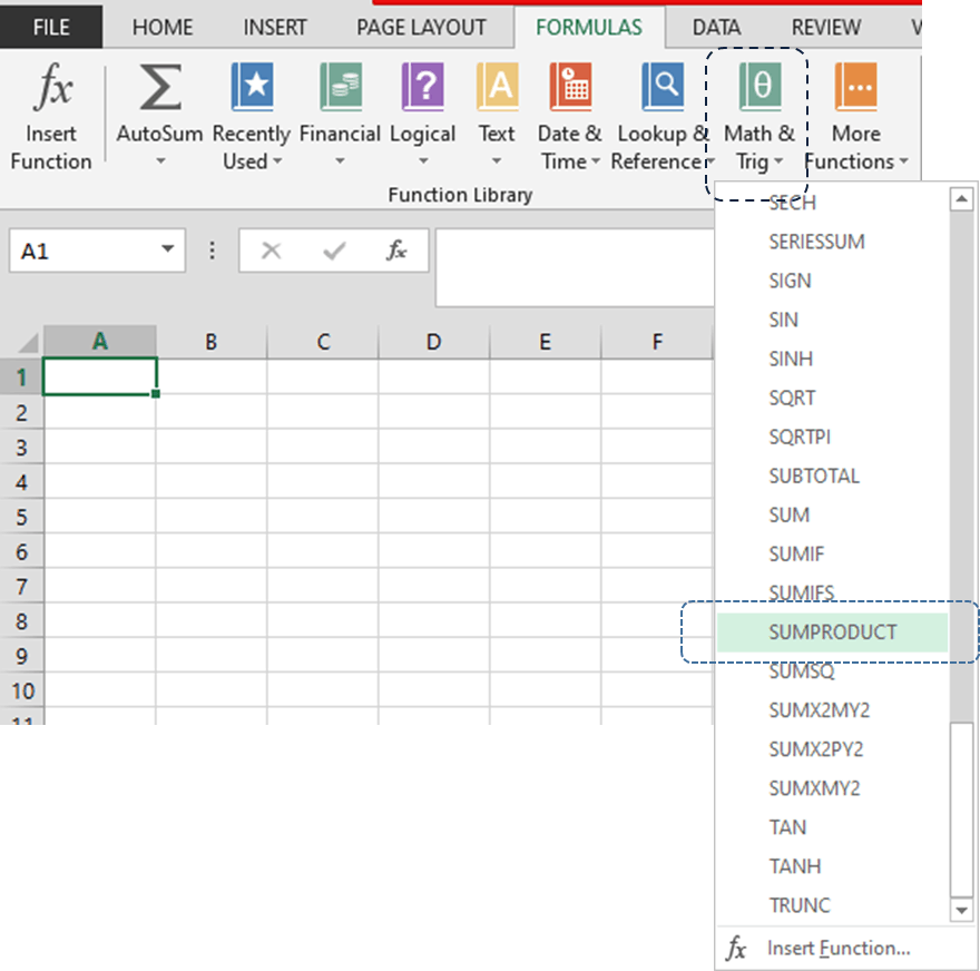
The SUMPRODUCT function in Excel basically has two steps:
Step 1: Multiply the range of cells or arrays (the default operation)
Step 2: All results from multiplication or products are summed up together
If you combine the two key keywords in step 2 (product and sum) you will come up with the SUMPRODUCT function in Excel. To understand these steps further, let’s take a look at the SUMPRODUCT formula below:
| Syntax of the SUMPRODUCT function in Excel |
| =SUMPRODUCT(array1,[array2],[array3],…) |

Where:
Array 1 A required argument representing a combination of rows and columns to be multiplied and summed up. The minimum number of arrays is 1.
[Array 2],[Array 3],… Optional arguments, the maximum number of arrays is 255.
For the SUMPRODUCT formula to work properly the Array 1,[Array 2],[Array 3],… must be
- Continuous,
- Have the same number of rows and columns, and
- Contain numeric values only (non-numerical values such as text or wildcard characters are treated as zeros).
To gain a good understanding of how to use SUMPRODUCT function in Excel, let’s go over its uses with examples.
Basic Use of SUMPRODUCT Function in Excel
This is our first stop in our journey to understanding how to use SUMPRODUCT function in Excel. Below is a list of 7 employees and their respective weekly hours worked and their hourly rate.
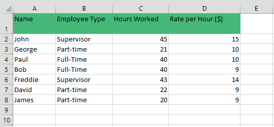
Form this table we need to know the Total Wages for the week. We calculate this by multiplying the hours worked (Column C) by their respective rate per hour (Column D) and then sum all the results or products to get the Total Wages.
You can use a simple approach similar to below, which results in $2,625 of Total Weekly Wages for All Employees.
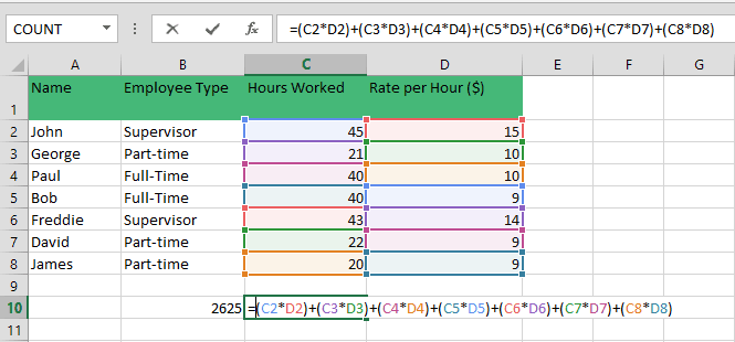
Alternatively, we can add a new column, Column E and name it Total Weekly Wage ($), reflecting the multiplication of the hours worked (Column C) by their respective rate per hour (Column D). Then use the SUM function in Excel to add all the products.
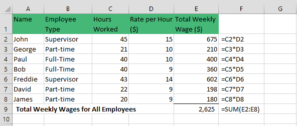
This results in Total Weekly Wages for All Employees of $2,625.
These two approaches gave us the same result but unfortunately, the process is lengthy and takes some time to input the formulas.
All these steps are simplified using the SUMPRODUCT function in Excel. The SUMPRODUCT formula =SUMPRODUCT(C2:C8,D2:D8) gives us a Total Weekly Wages for All Employees of $2,625.
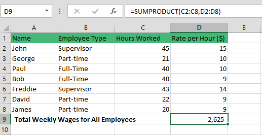
This is a basic example of how to use SUMPRODUCT function in Excel.
The SUMPRODUCT function in Excel performs the same mathematical operations as the previous approaches but calculates it quicker – imagine if you have a table with 20,30 or more rows!
The SUMPRODUCT formula’s array1 represented by (C2:C8) and array2 (D2:D8) multiplies the first number in the first column (C2) by the first number in the second column (D2) and so on and so forth. Once all rows or cells have been multiplied, the SUMPRODUCT formula automatically adds all results or products. It basically does the same mathematical process as our two previous calculations but a lot faster and requires lesser inputs.
Let’s move on to more advanced examples of how to use SUMPRODUCT Function in Excel.
How to Use SUMPRODUCT with One Criteria
Continuing on our journey, we will illustrate how to use SUMPRODUCT to multiply and sum ranges which meet the criteria. SUMPRODUCT function in Excel can be a conditional SUMPRODUCT, similar to a conditional SUM using the SUMIF function [link to SUMIF sub article].
Assume instead of calculating the Total Wages for All Employees, we want to know the Total Wages for Part-time Employees only. How to use SUMPRODUCT function in Excel?
The SUMPRODUCT formula =SUMPRODUCT(–(B2:B8=”part-time”),C2:C8,D2:D8) results in $588.
To double-check, we can identify the cells containing data for the part-time employees and use a simple formula =(C3*D3)+(C7*D7)+(C8*D8). This gives us a result of $588.
Let’s dissect the SUMPRODUCT formula to understand how to use SUMPRODUCT function.
| =SUMPRODUCT(–(B2:B8=”part-time”),C2:C8,D2:D8) |
Array1 represented by (–(B2:B8=”part-time”) acts as the filter or condition. It uses a logical expression to set the criteria that values in range (B2:B8) must meet – the Employee Type =“part-time” (do take note SUMPRODUCT formula is not case sensitive).
Filtering Column B for “part-time”, the result for Array1 is:
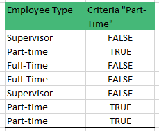
The array contains 7 values representing one for each row.
Since SUMPRODUCT function in Excel ignores non-numerical values, the TRUE/FALSE values must be converted numerically. The double negative ( — ), also called by its fancier name double unary operator, converts non-numerical values such as TRUE/FALSE values into its numerical equivalent 1/0.
Filtering Column B for “part-time”, the numerical result for Array1:
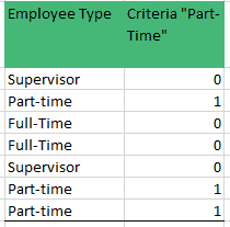
The number one (1) indicates a row where our criteria “part-time” employee matches and zero (0) indicates a row otherwise.
Array2 Represents the Hours Worked Column
Array3 Represents the Rate per Hour Column
To visualize the process (Array1 * Array2 * Array3), take a look at the table below:
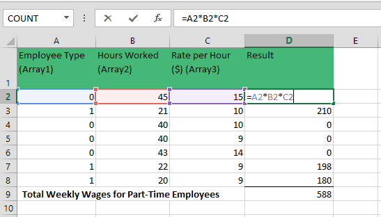
Which gives us a result of $588.
From our calculation, we can safely say that in certain circumstances the SUMPRODUCT function in Excel can replace the SUMIF function in Excel.
Now that we have illustrated how to use SUMPRODUCT function in Excel with one criterion, can we also use SUMPRODUCT with multiple criteria?
How to Use SUMPRODUCT With Multiple Criteria
Moving along our roadmap, aside from using one criterion we can use SUMPRODUCT with multiple criteria by simply expanding our arguments (SUMPRODUCT function in Excel accepts 255 arguments).
Continuing with our prior example, assume we want to know the Total Wages of Part-Time employees whose weekly working hour is greater than 20 hours.
Extending our SUMPRODUCT formula to add the second criteria; greater than 20-hours (>20). The new SUMPRODUCT formula is =SUMPRODUCT(–(B2:B8=”part-time”),–(C2:C8>20),C2:C8,D2:D8). This gives us a result of $408.
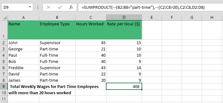
Array1 represented by (–(B2:B8=”part-time”) is still the 1st criterion that must be met, the Employee Type =“part-time”.
Array2 represented by –(C2:C8>20) is the 2nd and newly added criterion that also must be met, the Hours Worked greater than 20 (>20).
It is important to mention that Array1 and Array2 are following the AND logic. Both criteria must be met first before SUMPRODUCT function in Excel can work.
Array3 Represents the Hours Worked Column
Array4 Represents the Rate per Hour Column
To visualize the process (Array1 * Array2 * Array3 * Array 4), take a look at the table below:
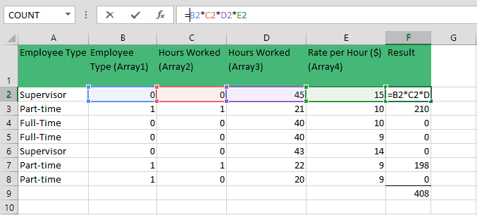
The number one (1) indicates a row where criteria1 “part-time” employee AND criteria2 greater than 20 (>20) matches and zero (0) indicates a row otherwise.
Using this example, we can safely say that in certain circumstances the SUMPRODUCT function in Excel can replace the SUMIFS function in Excel.
SUMPRODUCT Function In Excel Using OR Logic
So far our roadmap brought us to the different ways on how to use SUMPRODUCT – from the basic to SUMPRODUCT with multiple criteria and one criterion.
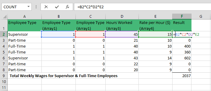
This portion will discuss one key strength of SUMPRODUCT function in Excel compared to other SUM functions. To illustrate, assume you want to know the Total Weekly Wages for both Supervisor and Full-time Employees.
If we use the same SUMPRODUCT formula for the SUMPRODUCT with multiple criteria, the SUMPRODUCT formula =SUMPRODUCT(–(B2:B8=”full-time”),–(B2:B8=”supervisor”),C2:C8,D2:D8) results in Zero.
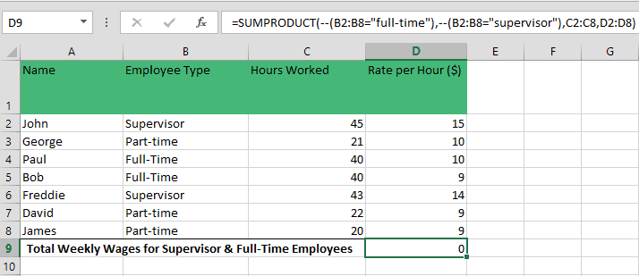
Why?
By design the SUMPRODUCT formula follows the AND logic, both criteria1 and criteria2 must be met or matched first before the SUMPRODUCT function in Excel works.
To solve Total Weekly Wages for both Supervisor and Full-time Employees, we need to apply the OR logic. To use the OR logic, we simply add the plus sign (+) to our criteria. The new SUMPRODUCT formula =SUMPRODUCT((B2:B8=”full-time”)+(B2:B8=”supervisor”),C2:C8,D2:D8) gives us $2,037.
To visualize the process (Array1 * Array2 * Array3 * Array 4), take a look at the table below:
SUMPRODUCT Function In Excel To Calculate Weighted Average
Weighted Average is an average resulting from the multiplication of each value by a factor representing its importance. From the definition alone, you can say the SUMPRODUCT function in Excel fits perfectly for this calculation as the SUMPRODUCT formula is designed to sum products.
Assume you conducted a quarterly performance review of one of your employees, below table are the performance grade and respective weights. To calculate the Weighted Average, we combine the SUMPRODUCT formula with SUM formula; =SUMPRODUCT(B2:B5,C2:C5)/SUM(C2:C5) results in 86.
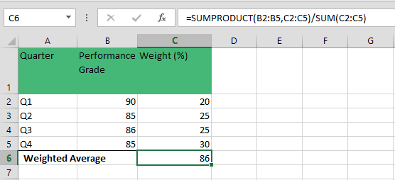
Array1 represented by (B2:B8) represents the Performance Grade.
Array2 represented by (C2:C8) represents the Weight (%).
The products of Array1 and Array2 are summed up and then divided by the sum of the Weights. Why?
If we only use the SUMPRODUCT formula =SUMPRODUCT(B2:B5,C2:C5) this gives us a result of 8,625. Which is the correct number but this is not what we are looking for. Dividing this by the SUM formula SUM(C2:C5), which results in 100, brings the number in line with the Performance Grades’ values.
Main Points From The Road Map On How To Use SUMPRODUCT
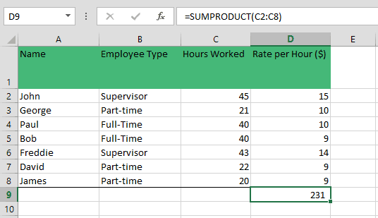
- SUMPRODUCT formula is designed to multiply then sum the products. If only one array is given, SUMPRODUCT function in Excel will only result in the total sum of the cells. To illustrate, assume instead of using =SUMPRODUCT(C2:C8,D2:D8), we only used Array1. The SUMPRODUCT formula =SUMPRODUCT(C2:C8). This gives us a result of 231.
- SUMPRODUCT function in Excel treats non-numerical values as zeros.
- When you use logical tests inside the arrays, these results in TRUE and FALSE values. Since SUMPRODUCT formula can only work with numerical values, use double negatives (–) to convert TRUE/FALSE results to 1’s and 0’s.
- SUMPRODUCT function in Excel can be used to conditional sum values with one and multiple criteria similar to SUMIF and SUMIFS functions.
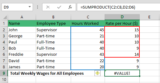
- Array arguments must have the same number of cells otherwise you’ll have a #VALUE! Error. SUMPRODUCT function in Excel accepts up to 255 arguments.
