The CEILING function in Excel is another way to round numbers in Excel. But unlike the ROUND functions, the CEILING formula in Excel has no rounding digit or decimal place to round to.

This article will help you understand what the CEILING function in Excel does, how to use the CEILING formula in Excel and, if it’s your first time using this function, the common errors you may encounter.

From the Ground Up with Excel’s CEILING Function

The CEILING function in Excel is one of the many ways to round numbers found in the Math/Trigonometry Formulas. You can round numbers using the conventional Math Rules or specifically round up or down.

Excel’s CEILING function is different from the other rounding functions because instead of focusing on decimal places, rounding digits and the number that follows or to the right of the rounding digit, the CEILING formula in Excel focuses on the nearest significant multiple.

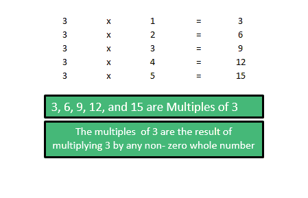
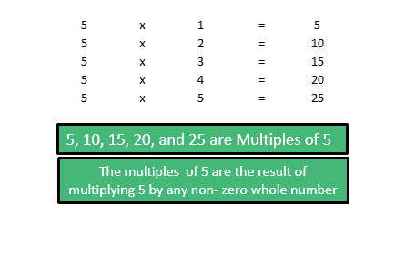
Recall in Basic Math class, a multiple is a result of multiplying a number by a non-zero whole number. The below table are basic examples of Multiples:

You might wonder why name this rounding function in Excel a CEILING function?

The answer is right under our nose, the CEILING function in Excel always rounds a number UP to nearest significant multiple and since the ceiling is always UP above us then it’s called the CEILING Function.

The CEILING formula in Excel:

Where:

Number – A required argument representing the number that has to be rounded. The Number argument can be positive and negative numbers, cell references, and formulas.

Significance – A required argument representing the multiple to round a number to e.g. multiple of 3, 5, etc. The multiple can have both positive and negative numbers and refer to cells.

Below are applications of the CEILING formula in Excel using the Multiples table we presented before:

• When both arguments have POSITIVE ( + ) signs, the CEILING formula in Excel rounds the number UP to the nearest multiple (see cells D2 and D3). Notice how the results round-up and away from zero.
• When both arguments have NEGATIVE ( – ) signs, the CEILING formula in Excel rounds the number UP to the nearest multiple (see cells D4 and D5). Notice how the results still round-up and away from zero.
• If the Number argument is NEGATIVE and Significance argument is POSITIVE, the CEILING function in Excel rounds a number UP to the nearest multiple but notice the result is rounded UP but towards zero (see cell D6).
• If the Number argument is POSITIVE and Significance argument is NEGATIVE the CEILING function in Excel results in a #NUM error (see cell D7)

Examples of How to Use Excel’s CEILING Function

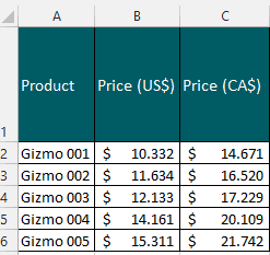
Assume a US-based manufacturing firm is planning to sell products in Canada and the management wants to determine how to price products in Canadian dollars (CA$).

Management’s course of action was to start with the US$ price and convert to CA$. But this approach results in prices that are quite different from the attention-grabbing prices we see (prices that end in 0, .99, .25, .75) and in essence leaves a little bit of money in the table.

Using Excel’s CEILING function we can round the CA$ prices up to multiple of 3s (CA$3), 5s (CA$5), 10s (CA$10). The CEILING formulas in Excel =CEILING(14.671,3) under the Product Gizmo 001 (Cell D2) in the table below rounds the number UP to the nearest multiple of 3 or CA$3 and results in CA$15.

The CEILING function in Excel can be used to round the prices to the nearest 25 cents multiple too. Using the same Product Gizmo 001, the CEILING formula in Excel =CEILING(14.671,.25) (see Cell D2) rounds the number UP to the nearest multiple of 25 cents or CA$.25. This results in CA$14.75.

If management decides to have a price that ends in .99, the CEILING function in Excel can still be used. Continuing with Product Gizmo 001, the CEILING formula in Excel =CEILING(14.671,1)-0.01 (see Cell D2) rounds the number UP to the nearest multiple of 1 or CA$1.00 (this gives us $15) and deducts .01 to give us CA$14.99.

Top Points To Remember Using Excel’s CEILING Function

• The #VALUE! Error occurs when one of the arguments CEILING formula in Excel is non-numeric.
• The #NUM Error occurs when:
  • If you’re using MS Excel 2010/2013 versions, when the Number argument is positive and the Significance argument is negative, the CEILING function in Excel returns #NUM error.
  • If you’re using MS Excel 2003/2007 versions, the Significance argument must have the same arithmetic sign (positive or negative) as the Number argument.

• Both the CEILING function in Excel and the ROUNDUP function rounds numbers UP. But the key difference is Excel’s CEILING function rounds to the nearest significant multiple while the latter rounds to the nearest digits or decimal places.
• Rounding does not happen in Excel’s CEILING function if the number is an exact multiple of significance. For example, rounding the number 5 to the nearest multiple of 5. CEILING formula in Excel =CEILING(5,5) will return the number 5.
• If you want to round numbers down with multiples, use the opposite of the  CEILING function in Excel and use FLOOR function instead.