In financial modeling and analysis, Excel tables are usually arranged vertically so when finding important values the VLOOKUP function is the go-to tool [VLOOKUP article]. But it is not uncommon for tables to be arranged horizontally and working with horizontal tables is not at all infrequent.

When searching for data arranged horizontally, the HLOOKUP in Excel is the go-to tool. The HLOOKUP function in Excel is the VLOOKUP function’s sibling which finds a value ROW-wise as oppose to COLUMN-wise.  In this article, we will discuss what The HLOOKUP function in Excel is and how different (or similar) it is to the VLOOKUP function. We will also guide you on how to use HLOOKUP Excel with examples.

Know The “H” in HLOOKUP On Excel

The HLOOKUP function in Excel is useful for finding values in rows (horizontal) from a table or range of cells. It searches a table’s 1^st or topmost row and returns an exact or approximate value in the same column based on a user-given row number.

To successfully use the HLOOKUP on Excel, the values to lookup must be on the top row. If an exact match is needed, the values do not have to be sorted. On the other hand, if an exact match found is not found and an approximate match is needed, the values must be sorted in ascending order (smallest to largest). When the HLOOKUP in Excel formula does not find either an exact or approximate match of the value to look up, it will return the #NA error.

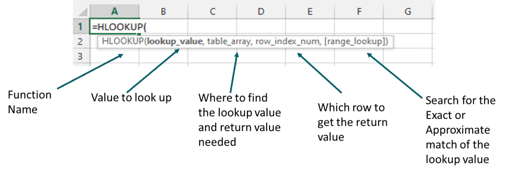
The formula for HLOOKUP on Excel:

Where:

Lookup_Value
– Represents the value to find which can be a numeric value, cell reference, or text string.
– If the Lookup_Value is a text string, wildcard characters (*) and (?) can be used.

Table_Array
– The range of cells where the HLOOKUP function in Excel will search from. (Required argument).

Row_Index_Num
– Represents the row number within the table_array to retrieve the data or return value needed (Required argument).
– The row number is relative to the range of cells selected or which row the horizontal table is presented in the Excel worksheet.
– A Row_Index_Num of 1 instructs the HLOOKUP in Excel formula to get the value in the 1^st row.
– A Row_Index_Num of 2 instructs the HLOOKUP in Excel formula to get the value in the 2^nd row.

[Range_Lookup]
– Defines whether HLOOKUP in Excel searches for an exact match or approximate match of the lookup_value (Optional argument).
– For an exact match, select False.
– For an approximate match, select True or simply omit.

5 Steps on How to Use HLOOKUP Excel

Step 1. Arrange Data Suitable for HLOOKUP in Excel

The HLOOKUP on Excel finds values horizontally or row-wise. For the function to successfully work, the values to lookup must be on the topmost row with the corresponding values to retrieve below. If finding an exact match, the data may or may not be sorted. However, for approximate matches, values on the topmost row must be sorted in ascending order (smallest to largest).

Step 2. Identify the 1^st required argument; the Lookup_Value

This step instructs Excel on what to look for. HLOOKUP in Excel can look up numbers, dates, names, and even wildcard characters.

Step 3. Define 2^nd required argument, the Table_Array

The 2^nd required argument directs the HLOOKUP on Excel formula where to find the Lookup_Value as well as the required return value by selecting the range of cells, named range, or table. The array can be on the same worksheet, a separate worksheet in the same workbook, or a completely different workbook.

Step 4. Specify Row Number from the Table_array

This step inputs the last of the 3 required arguments and specifies which row from the same column of the Lookup_Value to get the return value needed. Bear in mind the row number is relative to the range of cells selected and is user-defined. Similar to the VLOOKUP function, the HLOOKUP in Excel by itself cannot locate the row number.

Step 5. Choose between Exact (FALSE) or Approximate Match (TRUE)

This 5^th step is optional and instructs Excel to find an exact or approximate match of the Lookup_value argument. Despite being optional, this argument is important as selecting the wrong type will lead to different results. Omitting the match type has the same effect as selecting TRUE for an approximate match.

Examples on How to Use HLOOKUP Excel

HLOOKUP in Excel Example No. 1: Search Value for Exact Match

For this HLOOKUP in Excel example, refer to the below table reflecting the Euribor interest rates and the EUR/USD FX rate from 2^nd to 16^th of December.

How to use HLOOKUP Excel to find the Euribor interest rate for the 5^th of December.

1. Since this is a horizontal table where values to lookup are in the top row and the return values are below, the HLOOKUP function in Excel is a suitable function to use.
2.  The value to find or the Lookup_Value argument is the date 5^th of Dec. For this HLOOKUP in Excel example, instead of typing the Lookup_Value argument directly into the formula, we will use a reference cell. The reference cell is N2.
3. The range of cells or the Table_Array where to find the lookup value and return value needed is from cells B1 to L3.
4. The specific row or Row_Index_Num where to get the return value from the Table_Array is on the 2^nd row.
5. The lookup value must be an exact match so use FALSE for the [Range_Lookup].

Using the HLOOKUP on Excel formula =HLOOKUP(N2,B1:L3,2,FALSE), the Euribor interest rate for 5^th of December is -.269%

The HLOOKUP in Excel formula searches the top row of the Table_Array, cells B1 to L3, for the Lookup_Value 5^th of December. Once found, the formula then looks down (from the same column as 5^th of December) to the 2^nd row as specified by the Row_Index_Num argument. The HLOOKUP function in Excel then retrieves the corresponding return value of -.269%

HLOOKUP in Excel Example No. 2: Search Value for Closest (Approximate) Date

When an exact match cannot be found, HLOOKUP on Excel formula can also search for an approximate match. It is important to emphasize that the lookup values in the top row must be sorted in ascending order.  The HLOOKUP in Excel finds the next largest date that is lower than the lookup value.

Continuing with the example, find the EUR/USD FX rate for 7^th of December

1. The data is presented in a horizontal table with values to lookup in the top row and sorted in ascending order. The HLOOKUP function in Excel is a suitable function to use.
2. The reference cell for the Lookup_Value argument remains unchanged, reference cell N2.
3. The range of cells or the Table_Array where to find lookup value and the return value needed also remains unchanged, cells B1 to L3.
4. The specific row where to get the return value from the Table_Array is on the 3^rd row. Row_Index_Num is 3.
5. Since the return value is an approximate match, the [Range_Lookup] is TRUE or simply omit.

Using the HLOOKUP on Excel formula =HLOOKUP(N2,B1:L3,3,TRUE), the EUR/USD FX rate for the 7^th of December is $1.108.

Based on the dates on the top row, the 7^th of December is missing. Keep in mind the data is sorted in ascending order, so the HLOOKUP in Excel formula finds the next largest date that is lower than the Lookup_Value argument. The date that fits this condition and is considered as the approximate match is the 6^th of December. The function then looks down (from the same column as the 6^th of December) to the 3^rd row as indicated by the Row_Index_Num argument. The formula then retrieves the return value of $1.108.

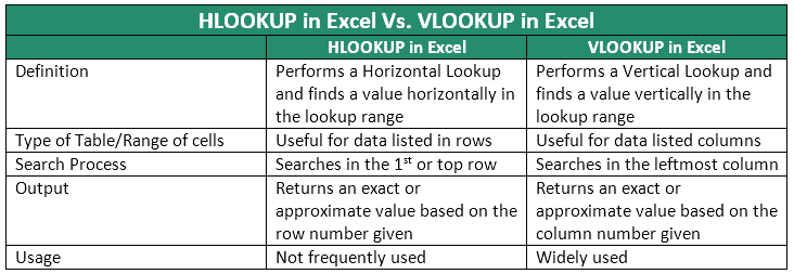
HLOOKUP on Excel Vs. VLOOKUP

The HLOOKUP function in Excel and the VLOOKUP functions are both part of the Lookup & Reference functions in Excel. Use the tables below to understand the similarities and differences between the two.

4 Key Points on How to Use HLOOKUP Excel

Remember below key facts when using the HLOOKUP on Excel to avoid incorrect results:

1. The HLOOKUP function in Excel searches in the 1^st or top-most row. If you need to look up a column, use the VLOOKUP function instead, or consider using Index & Match functions combined.
2. HLOOKUP in Excel is not case sensitive and does not distinguish uppercase and lowercase characters. Data containing duplicates poses incorrect results.
3. When searching for an approximate match, the lookup values in the top row must be sorted in ascending order.
4. The Row_Index_Num in the HLOOKUP in Excel formula must not be greater than the number of rows in the Table_array. If the range of cells has 3 rows, the row number must be from 1 to 3 only.