In this article, we will provide a brief overview of the major SUM Functions in Excel such as SUM, SUMIF, SUMIFS, and SUMPRODUCT Excel function. In financial modeling, SUM functions in Excel are frequently used. Let’s review the following four SUM functions in Excel and how they can be used for financial modeling purposes:

• SUM Function
• SUMIF Function
• SUMIFS Function
• SUMPRODUCT Formula

The SUM Function in Excel

In MS Excel, one of the most basic and commonly used formulas is the SUM Function. The SUM Function in Excel is a built-in function in Excel, categorized as a Math/Trig Function, and is used whenever you want to add up cell values. You can add up any numbers or refer to their cell addresses. The Syntax of the SUM formula in Excel is as follows:

SUM Function Syntax in Excel
=SUM(cell1, cell2, …)
=SUM(cell1:cell2,…)

Whereas:

• Cell1– the first cell address of the first. number to be included in the total
• Cell2– the second cell address of the number to be included in the total. This value is already optional.
• … – any additional value or cell address to be included in the sum as well.

Example SUM Formula in Excel
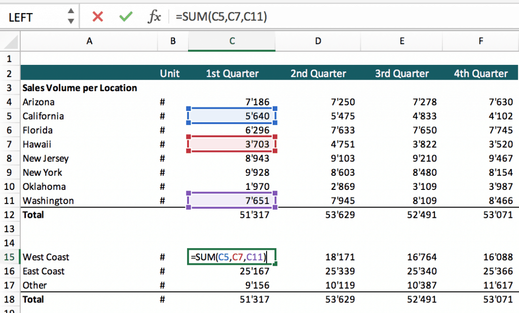
= SUM(C5,C7,C11)
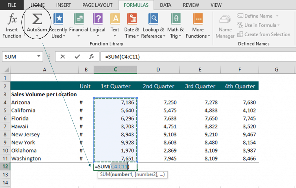
= SUM(C4:C11)

The first Syntax, adds up specific cells, while the second Syntax adds up a range of cells. Whenever Formulas in Excel use a comma (,), it means particular cells are referred to. Input Cell 1 and Cell2 are cell addresses in MS Excel, e.g., C5, C7, C11. Each address specifies the column and row number where the cell is located, which is the cell address (see above). The beauty of this is that each cell, C5, C7, C11 can include numbers, and by updating them, the SUM Function updates the total of the inputted figures by returning their updated total value.

When using a double point (:), it will include all cells starting from the first cell (top left) to the last cell (bottom right location in the Excel worksheet).

Here’s a summary of the key elements of the SUM Function in Excel:

KEY ELEMENTS of the SUM Function

• Purpose: Adding up numbers in Excel.
• Rationale: Dynamically calculate the total while you can update the input values separately.
• Number Format: The SUM Formula in Excel only works when numerical values are used. The SUM Formula will lead to errors if any form of text is included in the cell references.
• Maximum arguments: The SUM Function can add up to 255 arguments. The way to work around this limit is to use cell ranges. With cell ranges, a much larger number of cells can be added up (potentially up to the number of columns or rows).
• Empty Cells: Automatically ignores empty cells and cells with text values.

The arguments to be added in the SUM Formula can be numbers, arrays, cell references, constants, etc. To learn more about the SUM function in Excel, please refer to Microsoft’s official page.

The SUMIF Function in Excel

A particular case of the SUM Formula is the SUMIF Function in Excel. The SUMIF Function in Excel returns the sum of cells that meet a single logical criterion. To make this function work, the cells need to be arranged in a table format with a minimum of two columns and one criterion defined:

• Range – the first array of cells which can be filled with any attribute or label
• Criteria – defines the filter for which the range column shall be filtered
• Sum_range – contains the numbers which shall be included in the addition provided their corresponding range value meets the defined criteria

SYNTAX SUMIF Function in Excel
=SUMIF(Range, Criteria, Sum_range)

Example SUMIF Formula in Excel
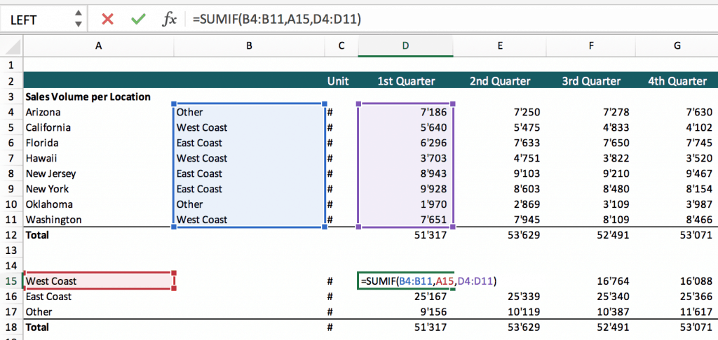
= SUMIF(B4:B11,A15,D4:D11)

Important to note is that the SUMIF Function is mostly used with cell ranges. E.g., opposite to the previous example, we don’t have to select cells such as C5, C7, C11 manually anymore, we can automate the task. We add another column which specifies the region of each state; then, we tell Excel only to sum up those states which match the desired region. If we put a single cell value as criteria, it means we only add up those cells where column B equals the selected criteria (West Coast in the below example). Mainly, when there are many changes in a financial model, the SUMIF Formula saves us from a lot of manual work when having to update sub-calculations which are only focused on a subset of the total.

Possible criteria for the SUMIF Function can be any of the following:

• Cell references, e.g. criteria = C2. In this case, only numbers are added up if the value in the range cell is equal to the defined criteria.
• Logical operators, e.g., criteria =”>2″ will add up cells only where the cells in the ranges are greater than 0. You can use any logical operators such as >,<,<>,=, or also combine them with the cell values.
• Combinations between logical operators and cell references: e.g.criteria = “>”&C2. Combinations are characterized by the use of &, combining multiple cells or values.
• Wildcards: e.g., criteria “*a” where the second letter is an a.

KEY ELEMENTS of the SUMIF Function

• Purpose: Adding up numbers in Excel which meet the defined criteria
• Rationale: Automates calculations that are only interested in a subtotal rather than the full total.
• Number Format: Same as the SUM Function, the SUMIF Formula in Excel requires that the sum area is inputted in the form of numbers only. However, values in the range array and criteria do not need to be ‘numbers’.
• Maximum arguments: The SUMIF Function only allows one to enter one criterion. If you need to filter your list for more than one criteria, use the SUMIFS Function.
• Empty Cells: Only cells meeting specific criteria are added. Therefore, empty cells become irrelevant.

To learn more about the SUMIF formula in Excel, please see also Microsoft’s official explanation here on the SUMIF formula or refer to this article: How to use the Excel SUMIF formula.

SUMIFS Function in Excel

The SUMIFS Function in Excel works similarly to the SUMIF Function but now we can add multiple criteria instead of using just one criterion. Same as the SUMIF formula, the SUMIFS function in Excel requires to arrange all values in a table format. The syntax for the SUMIFS Formula is as follows:

SYNTAX of SUMIFS Function in Excel
=SUMIFS(Sum_range, criteria_range1, criteria1, criteria_range2, criteria2, …)

Whereas:

• Sum_range – refers to the range of cells to be added together. Please note, opposite to the SUMIF function, the SUMIFS function puts the cell range to be added up together first in the Syntax of the function.
• Criteria_range1 – refers to the range of cells, which include the argument for condition1.
• Criteria1 – refers to the first condition which needs to be met to add up the corresponding number in the Sum_range.
• Criteria_range2 – refers to the range of cells, which include the argument for condition2.
• Criteria2 – is the second condition that needs to be met as well to add up the corresponding number in the Sum_range. Please note, criteria 2 is already optional.
• Criteria_range3 …
• Criteria3…

Example SUMIFS Formula in Excel
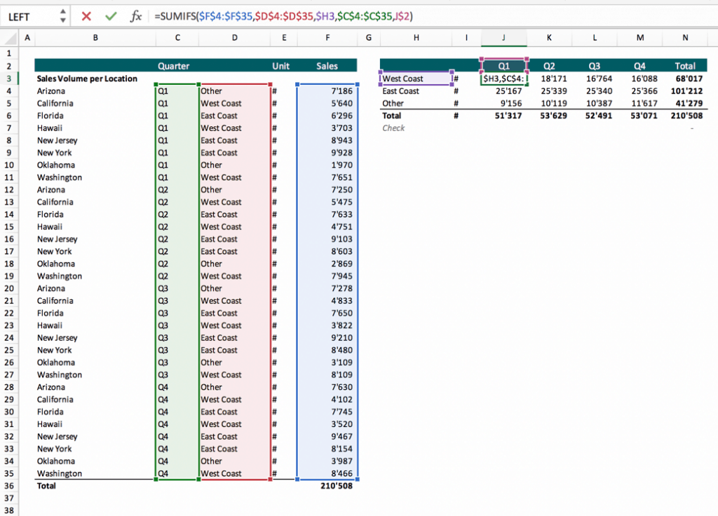
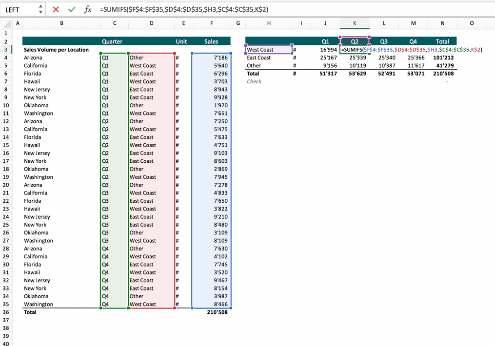
=SUMIFS(F4:F35,D4:D35,H3,C4:C35,J2)

The following screenshots show an example of the SUMIFS Formula in Excel. Please note, the $ sign is added so that when you copy the formula to another cell, the cell addresses remain fixed. If you remove the $ signs, the array would be shifted as well (to the right and to below) when copy/pasting this formula to a different cell.

KEY ELEMENTS of the SUMIFS Formula

• Purpose: Adding numbers in Excel which meet multiple criteria.
• Rationale: Allows to calculate detailed breakdowns from an extensive data set by extracting the subtotal which meets multiple criteria.
• Number Format: Same as the SUMIF Formula, the SUMIFS Formula in Excel requires that the sum area is inputted in the form of numbers. Criteria_range and criteria do not need to be ‘numbers’ and can be ‘text’.
• Maximum arguments: The SUMIFS Function can handle up to 127 criteria pairs. In reality, only a few criteria will be used as you would require an extraordinary large dataset to use 127 criteria, which generally is not the case in financial modeling applications.
• Empty Cells: Empty cells are irrelevant as either the criteria are met or are unmet.

The SUMIFS function was a function only added in later versions of MS Excel to make it easier for users to include additional criteria. To learn more about the SUMIFS function, please also refer to Microsoft’s page about the SUMIFS function in Excel.

The SUMPRODUCT Formula

The SUMPRODUCT Formula allows you to multiply numbers in two or multiple arrays together and then add up their totals. The function is mainly used to avoid a step by step calculation and get to the total in one single shot, therefore speeding up calculations in an elegant way:

SYNTAX SUMPRODUCT Formula in Excel
=SUMPRODUCT(array1, array2, …)

Whereas,

• Array1 – the first cell array containing numbers
• Array2 – the second cell array containing numbers to be multiplied with the figures included in Array1
• Array… – any additional cell arrays to be included in the multiplication

Example SUMPRODUCT Function in Excel
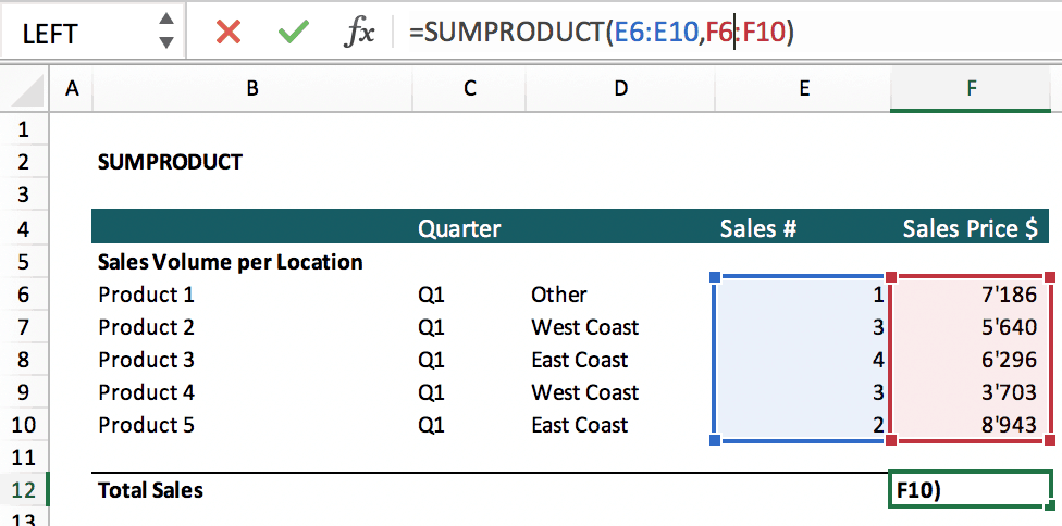
=SUMPRODUCT(E6:E10,F6:F10)

The following examples show a table containing the number of sales and the sales price. The SUMPRODUCT formula allows you to calculate the total of all multiplied numbers in one go.

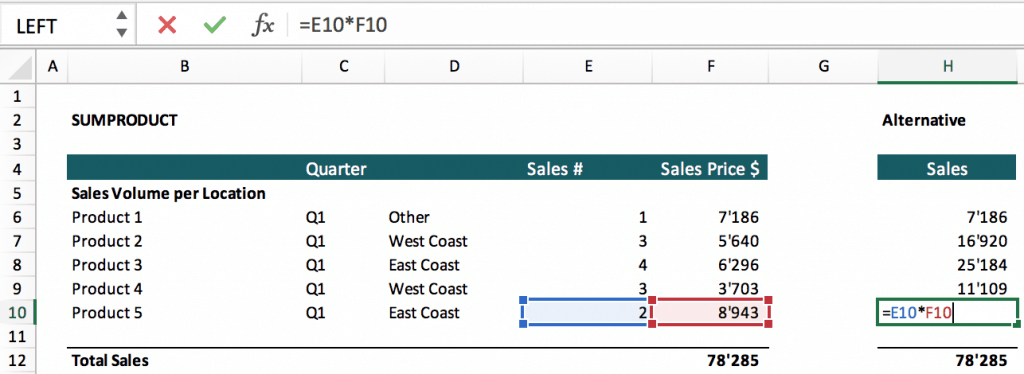
However, in financial modeling, the SUMPRODUCT formula many times is not used as its challenging to understand and to check if the result is correct or not. E.g., if some of the cells are entered as text and not as numbers (entering ‘8943 instead of 8943), the result will not be correct. To avoid this problem, many times financial modelers prefer to do a step by step calculation, first applying the multiplication on a separate column and then merely adding up the multiplied numbers. The result is the same; the only difference is that the alternative formula is easier to audit than the SUMPRODUCT Formula.

KEY ELEMENTS of the SUMPRODUCT Formula

• Purpose: Multiplies arrays of numbers in Excel and sums up their total
• Rationale: Speeds up calculations where otherwise step by step calculations would be needed (first multiplication, then second the addition of the multiplication results).
• Number Format: All the figures included in the arrays need to be entered as numbers.
• Maximum arrays: You can include up to 255 arrays with the SUMPRODUCT Formula.
• Empty Cells: Are treated as zero. Therefore, multiplication and total lead to zero until it is corrected.

Comparison of all SUM Functions in Excel – SUM, SUMIF, SUMIFS, and SUMPRODUCT

What does it do?
SUM – Adding up numbers
SUMIF – Adds numbers if they meet specific criteria
SUMIFS – Adds numbers if they meet multiple criteria
SUMPRODUCT – Sums up the multiplication of numbers which are multiplied across an array

Rationale
SUM – Calculating the total
SUMIF – Calculating a Subtotal
SUMIFS – Calculating subtotals of a large data set
SUMPRODUCT – Perform a two-step calculation (multiplication followed by an addition) in one go

Use Cases
SUM – Addition of select values/cells and Addition of cell ranges
SUMIF – Creating breakdowns of data and Extracting summaries from large data sets
SUMIFS – Creating more detailed breakdowns of Data and Extracting more detailed summaries from large data sets
SUMPRODUCT – One-step multiplication + addition (instead of two-step calculation)

Number format
SUM – Required
SUMIF – Only the cell array containing the numbers to be added up
SUMIFS – Only the cell array containing the numbers to be added up
SUMPRODUCT – Required

Empty Cells
SUM – Excluded. If numbers are entered as texts, they will not be added in the total
SUMIF – Irrelevant
SUMIFS – Irrelevant
SUMPRODUCT – Are treated as zero, need to contain numbers

Maximum Number of Arguments
SUM – Up to 255 components to be added together
SUMIF – 1 argument
SUMIFS – 127 arguments
SUMPRODUCT – 255 arrays

SUM Functions in Excel – You will need them!

It is undeniable that the SUM Functions in Excel offer beneficial applications, not only for summing up simple numbers with the SUM Formula but with the SUMIF and SUMIFS Formula also for filtering more massive data sets, calculating subtotals to obtain more insights and a deeper understanding on the composition of a total calculation.

• SUM Formula helps to add up numbers dynamically as per the inputted cell values.
• SUMIF Formula adds up numbers meeting one criterion
• SUMIFS Function adds up numbers which need to meet multiple criteria
• SUMPRODUCT Formula adds up the multiplication of numbers arranged in an array

Overall, these formulas are found in many, if not most financial model templates and therefore are essential to understand for financial modeling purposes.