The SUM function simply adds all numbers in a range of cells and is one of the most basic and widely used built-in functions in Excel. In this tutorial, we will discuss scenarios why the SUM function in Excel is not working and other errors in Excel you encounter when using this function.

Let us look into 5 essential points on how to use SUM function in Excel properly and how you can benefit the most from this basic function.

No.1 I Inserted A New Row But SUM Function In Excel Is Not Working

This is a basic example of how to use the SUM function in Excel properly. Not understanding the limitations of the SUM function in Excel can lead to misstatements in your financial data.

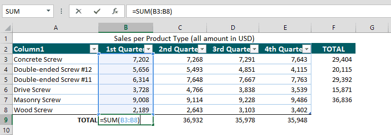
A manager at a leading industrial company has below Quarterly Sales Table.

The company manufactured a new product, Wood Screw. To update the table he inserted a new row above the row Total (Column A) and entered its respective Quarterly Sales.

But he noticed the SUM function in Excel is not working correctly as it ignores the newly inserted row, the SUM formula in Excel =SUM(B3:B7). In other words, the original reference cells were maintained and row for the new product was not ignored.

What does this error in Excel in the Sales Table mean? For one, the company’s Total Sales are grossly understated. Sales forecasts based on historical data will also be adversely affected.

How about inserting a new column in the table? The same error happens with a newly inserted column (Column F) at the left of Total (Column G), the SUM formula in Excel =SUM(B3:E3). The SUM function in Excel is not working properly as it maintained the original range of cells.

How to use SUM function in Excel in this case and avoid this costly error in Excel?

You can simply edit the SUM function in Excel by expanding the range of cells using “drag and drop” to include the inserted row and column. But you will be repeating this step every time you add a new row and column. If your data is not complex this step may not be cumbersome.

But how to use SUM function in Excel if you’re dealing with a large amount of data?

You can convert the range of cells into a table. To convert a set of data into a Table:

1. Click inside the data set.
2. On the Insert tab, click Table in the Tables group.
3. Specify if the table has headers or not. In this case, the data set has headers.
4. Click OK.

When you insert columns and rows in the table, the references will update automatically. This solves the issue of the SUM function in Excel not working as it should be.

No. 2 SUM Function In Excel Is Not Working And Results In 0 (ZERO)

Excel and its many functions is a powerful tool to sort and analyze financial data but this is highly dependent on how you input data.

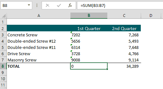
SUM function in Excel is not working because the reference cells are not number-formatted, meaning cells are text-formatted. If you instruct Excel to use the SUM function, then it rightly assumes the cell has numeric values. At times, data copied or imported to the worksheet (.csv files for example) are formatted as text. How can you tell if the cells are number-formatted vs. text-formatted?

The simple answer is knowing your right from your left. By default, text data is left-aligned while number data is right-aligned. Another clue to let you know of this type of error in Excel is the green flag appearing on the leftmost corner of each cell.

How do you convert text data to number format to avoid this error in Excel? Convert text into number by changing the cell format.

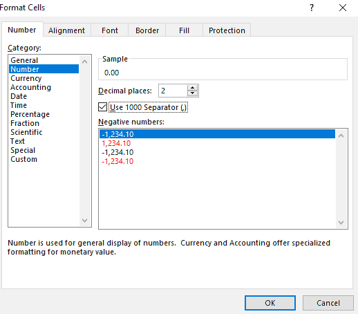
• Select the cells with text-formatted numbers.
• On the Home tab, in the Number group, choose General (default number format in excel, displayed just the way the user types it) or Number from the Number Format drop-down list.

Supposing the numbers are already formatted correctly but still the SUM function in Excel not working as it should and results in Zero (0). A circular reference is a common cause of this problem. A circular reference happens when a formula refers back to its own cell, think of as forming a loop. But fret not as excel gives you a heads up when this happens.

No.3 SUM Function In Excel Is Not Working And Results In #REF! Error

The #REF error in Excel is perhaps one of the most challenging in excel. The REF is short for “reference” and is displayed when the reference cell no longer exists. The missing reference cells are usually caused by mistakenly deleting the reference cells. Another reason is when the reference cells are Relative References (as opposed to Absolute References). By default all cell references are relative references, it is relative because when these are copied to a new cell it changes based on the position of the cell of the rows and columns.

For example, the table below has been updated to reflect the Total Sales in the first half (H1) and the second half (H2) for the year.

The #REF error in Excel appears when the 2^nd quarter sales column is removed.

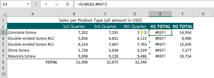
The #REF error in Excel also appears if the formula for the H1 Total Sales under Concrete Screw is copied and pasted to a new cell (B10) since the reference cells are relative reference the formula changes and moves depending on the cell location (B10).

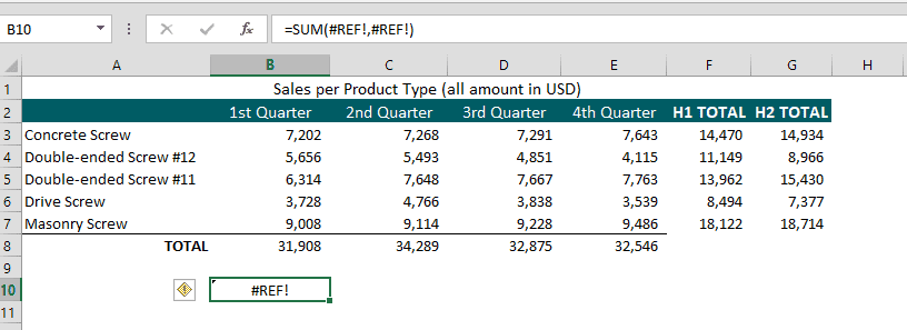
How to use SUM function in Excel to avoid the #REF error in Excel?

For the missing references, detect the #REF! error in Excel inside the SUM formula. Then replace the #REF! to the updated or correct reference cell or range.

For the Relative References, simply convert to Absolute References by “Locking” the cell. A cell is locked by inserting a dollar sign ($) into the formula. The SUM formula shows =SUM($B$3:$C$3)

No. 4 How To Use SUM Function In Excel To Reflect The Running (Cumulative) Total?

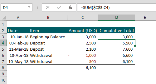
A running or cumulative total is simply the total number or amount of a sequence of numbers. The running total changes or updates as you continue to add (or subtract) the sequence, its main purpose is to show the total at any point in time. This is common in everyday use such as a store’s cash register, inventory system, a bank account’s deposits, and withdrawals, an amortization schedule showing loan due and the amount paid, etc.

A small business owner who knows how to use SUM function in Excel can use it for record-keeping.

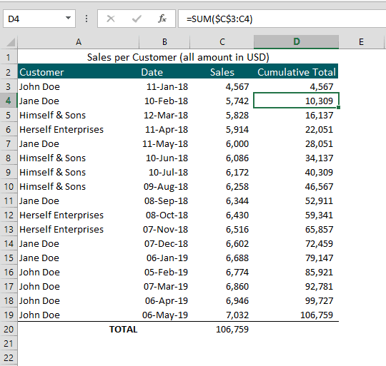
In our above example to calculate the cumulative total in Column D starting with Cell C4, we use the SUM formula =SUM($C$3:C4).

The 1^st reference cell must be absolute ($C$3), it should always refer back to Cell C3.

The 2^nd reference cell is relative (no $ sign) so it adjusts to the cell position where the formula is copied and pasted.

When the SUM formula is copied and pasted to Cell D5, it will be =SUM($C$3:C5) and adds Cells C3 to C5.

An individual who understands how to use SUM function in Excel can use also it for budgeting.

No. 5 How To Use SUM Function In Excel As A Conditional Sum

Aside from the common SUM function, a user can instruct Excel to add numbers given a certain parameter or condition. For example, you can instruct Excel to sum values if these are greater than, less than or equal to your own set of criteria. The SUMIF function also referred to as the conditional sum, does exactly this.

The SUMIF function has 3 arguments, the first 2 are required and the 3rd is optional.

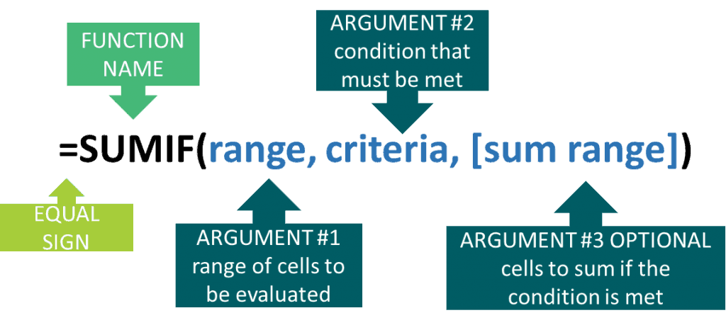
To illustrate the SUMIF function, let us use the table below to calculate how much sales the business earned from each customer.

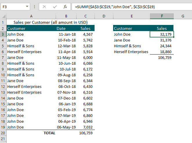
Delve deeper with more business examples and scenarios on how to use SUMIF and SUMIFS functions in Excel.

3 Bonus Tips on How to Use SUM Function in Excel

A few more reasons and solutions on SUM function in excel not working and how to avoid it that is worth to mention.

#NAME Error In Excel Appears Instead Of The Expected Result

This is the easiest and quickest way to fix. 99% of the time you encounter this error in Excel because of a simple misspelling. If you learned how to use SUM function in excel by manually entering the =SUM function instead of using AUTOSUM, chances are you may have misspelled SUM at some point in time. Read on the two ways on how to use SUM function in Excel.

SUM Function in Excel Not Working And Not Updating

If you have already entered the updated values but the totals continue to reflect the old values, most likely the excel worksheet’s Calculation Mode is set to Manual. This is not necessarily an error in Excel but is commonly encountered. To fix this,

1. Go to the Formulas tab,
2. Click the dropdown arrow next to calculate Options; and
3. Click Automatic.

The Automatic calculation will re-calculate the worksheet when a value changes or based on specific actions by the user such as inserting, deleting, hiding rows or columns, or renaming a worksheet.

SUM Function In Excel Not Working And Reflects Higher Number Than Expected Result

For more effective analysis of financial data, a user may need to filter or hide some data in the worksheet. How to use SUM function in excel correctly in this scenario is to understand that the SUM function adds all values in the specified range including both hidden (filtered) and visible cells.

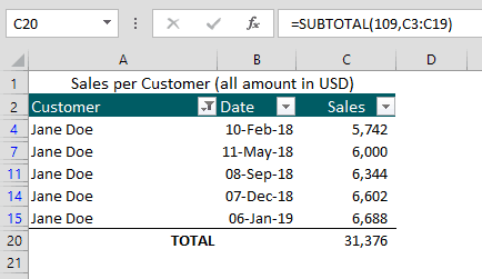
To illustrate, the sales table below is filtered by the customer “Jane Doe” and all other customers are hidden. But notice the TOTAL reflects the sum of all cells in the range both hidden and visible, essentially higher than expected.

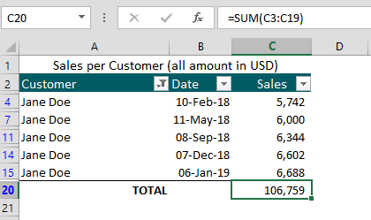
This is not necessarily an error in Excel but can be considered as a limitation of how to use the SUM function in excel. To fix this, use instead the SUBTOTAL function to sum the filtered data in Excel.

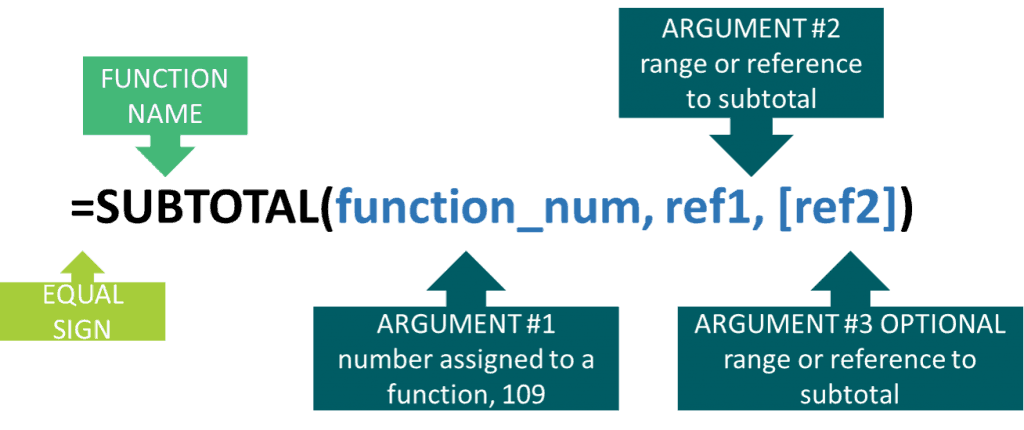
Take note that function_num is a number that specifies the function to use in calculating subtotals within a list and is already pre-assigned by Excel.