Up, Up, and Away with ROUNDUP Function in Excel

The ROUNDUP function in Excel doesn’t necessarily follow the conventional Math rules on rounding numbers. All numbers are rounded up, so the values resulting from using the ROUNDUP formula in Excel are always larger than the non-rounded or original number.

In this article, we will go through how to round up numbers in Excel by learning what  ROUNDUP function in Excel is, what essential parts are required in the ROUNDUP formula in Excel, and examples on how to use it.

The Way Up with ROUNDUP Function in Excel

The ROUNDUP function in Excel is 1 of the 3 ROUND functions under Math/Trigonometry you can use to round numbers in Excel.

This function does not follow the general Math rules for rounding numbers, it doesn’t round a number either up or down to a specific number of digits based on the number to the right of the rounding digit similar to what the ROUND function does.

Normally, the rounding digit is considered as the least significant digit and gets changed depending on the number following it (to the right of it). However, using the ROUNDUP function in Excel regardless of the number following the rounding digit is either 1,2,3,4,5,6,78, or 9, it will always be rounded up by 1 digit or the nearest 10s,100s, etc.

The syntax of the ROUNDUP formula in Excel:

Where:

Number – Required argument that represents the number that has to be rounded. You can use numbers (positive + and negative – signs), reference cells, and formulas.

Num_digits – Required argument that represents the number of digits to round the number to. You can reference the number itself or a reference cell.

• If the Num_digits is greater than zero it rounds a number in Excel UP towards the RIGHT of the decimal point- tenths, hundredths, thousandths, etc. (See cells D2 and D3 in the table below)

• If the Num_digits is zero it rounds a number in Excel UP towards its nearest integer or whole number. (See cell D4)

• If the Num_digits is less than zero it rounds a number in Excel UP towards the LEFT of the decimal point – ones, tens, hundreds, etc. (See cells D5 and D6)

One key point to remember on how to round up numbers in Excel using the ROUNDUP function is it can be used for numbers with positive ( + ) or negative ( – ) signs. For example, assume a business suffered a loss of -$1,130.143. You can use the ROUNDUP function in Excel however notice how the losses rise depending on the Num_digits argument used. Keep in mind, the ROUNDUP formula in Excel always rounds up, up, and away from zero.

Examples of How to Use ROUNDUP Function in Excel

The ROUNDUP function in Excel is simple to use and versatile, you can use it with other functions and formulas.

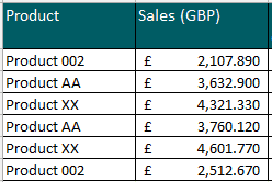
Assume a US-based business sells its products to the UK market, the table below is its GBP denominated sales.

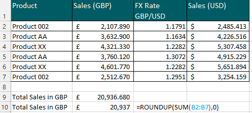
Using the ROUNDUP function in Excel, you can round the conversion of each GBP to USD sales.

As you can see, you can incorporate formulas (add, multiply, divide, etc.) in the Numbers argument in the ROUNDUP formula in Excel. For example under Product 002, the Numbers argument multiplies Sales GBP (cell B2) by FX Rate (cell C2). The Num_digits rounds the result up to 2 decimal places which give us a rounded sales figure of $2,485.42

ROUNDUP function in Excel can also be combined with other Excel functions.

You can combine ROUNDUP formula in Excel with the SUM function to round up the Total Sales in £ and US$ currencies.

Using the ROUNDUP formula in Excel =ROUNDUP(SUM(B2:B7),0) results in a Total Sales in £ of 20, 937. The formulas have a 2-step process:

1. Sums all Sales in GBP (B2:B7) which totals at £20,936.680 then
2. Rounds up the total sales value to its nearest whole number resulting in a Total Sales of £20,937.

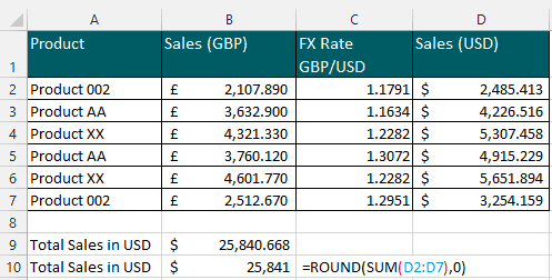
Applying a similar ROUNDUP formula in Excel for the US$ currency.

Critical Notes on ROUNDUP Function in Excel

• The ROUNDUP function in Excel always rounds a number up and away from zero and does not follow the conventional Math rules on rounding numbers.
• The Numbers argument in ROUNDUP formula in Excel works with numbers, cell references, and Excel formulas and functions.
• If you want to round numbers using conventional Math rules, use the ROUND function in Excel
• If you want to round numbers down or the total opposite of ROUNDUP function in Excel, use ROUNDDOWN function in Excel
• The ROUNDUP formula in Excel works for numbers with either positive ( + ) or negative ( – ) signs and can round either to the left or right of the decimal point.

Lovenna Tibas Store Manager

Lovenna Tibas is the Store Manager at eFinancialModels, specializing in website management, platform optimization, and customer support. She also writes about financial modeling topics including business valuation and business models, making complex concepts accessible to readers. With expertise in WordPress, Easy Digital Downloads, and e-commerce troubleshooting, Lovenna combines technical skills with a deep understanding of financial principles. Her work focuses on helping businesses leverage digital tools and financial insights to drive growth and make data-driven decisions.

See Full Bio

Excel Financial Modeling General Excel Financial Models