The COUNTIFS function in Excel with multiple criteria gives a lot of elbow room to pinpoint details important for analysis and financial modeling by using additional key metrics or criteria. In this essential guide, we will go over the basics of this Excel statistical function, understand its different parts and using examples for you to follow.

An Excel Statistical Function That Stripped Down the Basics

COUNTIFS function in Excel is a built-in function under the Statistical Function category. It applies a set of criteria to cells covering multiple ranges and counts the number of cells that match all the criteria. The result is always a numerical value.

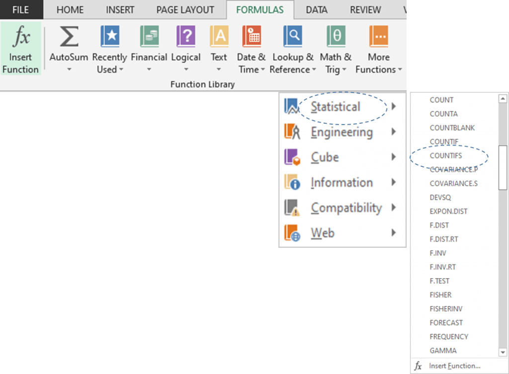
The COUNTIFS formula in Excel

Where:

• Criteria_Range1. The range of cells that will be tested against Criteria 1.
• Criteria1. The defined condition each of the cells in a Range1 is tested against.
• Criteria_Range2. The second (optional) range that will be tested against Criteria2.
• Criteria2. The second (optional) criteria to use on Range2.

This Excel statistical function with multiple criteria allows each criterion to be expressed as any of the following:

1. Numbers, Dates, and Time (10, 15/01/2018)
2. Text (“Sales”, “Cost”, etc.)
3. Cell Reference (A1, B1, C1)
4. Logical Operators <,>,<>,= (“>10”, “>=20”)
5. Wildcard characters (*,?). A question mark (?) matches any single character and an asterisk (*) matches any sequence of characters.

Each of the range’s criteria is applied to one cell at a time. If the first cell meets its respective criteria, the count goes up by 1. If the second cell meets its respective criteria, the count goes up by 1 again, and so on and so forth until all of the cells are tested against their respective criteria.

Another way to look at it is through multiple criteria that takes all of the Criteria_Range1, Criteria1 pairs and counts only those occurrences where all of the pairs are true or matches.  This Excel statistical function allows up to 127 Criteria_Range1, Criteria1 pairs. This makes it a robust and reliable tool to filter your data according to your specifications.

What are the Key Differences Between COUNTIFS and COUNTIF Functions in Excel?

Also, don’t miss learning with examples when using the COUNTIF function in Excel in this article: How to Use COUNTIF Function in Excel.

Learn the 5 easy ways to COUNT in Excel by reading this article: How to Use Count Functions in Excel.

By default, this Excel statistical function is designed to match ALL the multiple criteria before cells are be counted. It follows the ‘AND’ logic.

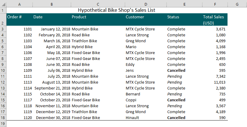
Here are examples of these multiple criteria, we will use a hypothetical bicycle store’s Sales List below.

By default, the COUNTIFS function in Excel is designed to match ALL the multiple criteria before cells are be counted. The COUNTIFS function in Excel follows the ‘AND’ logic.

Here are examples of COUNTIFS function in Excel with multiple criteria, we will use a hypothetical bicycle store’s Sales List below.

Example Using Multiple Text Criteria

Suppose you want to count the number of cells containing Mountain Bikes AND under Complete Status. In that case, you can use the Formula Syntax: =COUNTIFS(B3:B18, “mountain bike,” D3:D18, “complete”), which will give you a total count of 1 (as it count blank cells if another cell meets criteria).

You can breakdown the COUNTIFS formula in Excel as follows:

• Range1. Cell range C3:C18 are the cells that will be tested against Criteria 1.
• Criteria1. “mountain bike”  is the defined condition each of the cells in a Range1 is tested against.
• Range2. Cell range E3:E18 is the second range of cells that will be tested against Criteria2.
• Criteria2. “complete” the second criteria to use on Range2.

Notice that the range of cells is different C3:C18 and E3:E18. This is one of the key advantages of COUNTIFS function in Excel over the COUNTIF function. The same or different ranges can be used in the COUNTIFS formula in Excel.

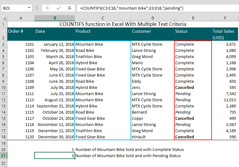
Another similar example is counting the number of cells containing Mountain Bikes AND under Pending Status. The COUNTIFS formula in Excel =COUNTIFS(C3:C18,”mountain bike”,E3:E18,”pending”) results in a total count of 3.

As you notice, the COUNTIFS formula in Excel is not case sensitive. So, typing “mountain bike” or “Mountain Bike” will still give a total count of 3.

Example Using with Wildcard Characters

In the real world, details in your data are not entirely unique. Data can have different versions and may contain similar characters. You can use the following wild characters to filter your criteria.

• Asterisk (*) – matches any one or more characters. This is used when counting cells containing a specific word or a character(s).
• Question mark (?) – matches any single character. This is used when counting cells beginning and/or ending with certain characters.

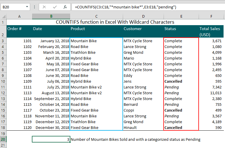
To illustrate, assume the Mountain Bike has a second version, simply called Mountain Bike v2. If you want to count the number of cells containing Mountain Bikes regardless of any version, use the Asterisk (*) in your COUNTIFS formula in Excel.

Continuing with our prior example, so to count the number of cells containing Mountain Bikes regardless of any version AND under Pending Status, the COUNTIFS formula in Excel =COUNTIFS(C3:C18,”*mountain bike*”,E3:E18,”pending”) will give us a total count of 3.

Example Using Multiple Number Criteria

This Excel statistical function is very useful in counting cells between two numbers like counting the number of cells that fall within determined limits (minimum and maximum) or boundary.

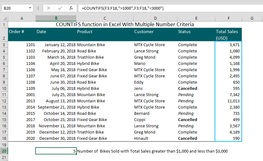
Assume you want to count the number of cells in the Total Sales column containing a number between $1,000 (minimum) and $3,000 (maximum) boundary.

The COUNTIFS formula in Excel =COUNTIFS(E3:E18,”>1000″,E3:E18,”<3000″) results in a total count of 5.

A breakdown of the COUNTIFS formula in Excel:

• Range1. Cell range F3:F18 is the cells that will be tested against Criteria 1.
• Criteria1. “>1000” is the defined condition each of the cells in a Range1 is tested against.
• Range2. Cell range F3:F18 is the second range of cells that will be tested against Criteria2.
• Criteria2. “<3000” the second criterion to use on Range2.

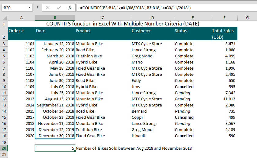
A similar example is using COUNTIFS function in Excel to count cells between two Dates.

Assume you want to count the number of cells containing dates between Aug 1 to Nov 30. The COUNTIFS formula in Excel =COUNTIFS(B3:B18,”>=01/08/2018″,B3:B18,”<=30/11/2018″) gives you a total count of 5 (as it count blank cells if another cell meets criteria).

5 Takeaways on COUNTIFS Function In Excel

1. The beauty of this Excel statistical function is there is no need for you to sort your list, it is very useful for the UNSORTED list.
2. It is designed to apply the ‘AND’ logic across various sets of criteria given.
3. Its Formula Syntax: Criteria_Range2, Criteria2… pairs must have the same number of rows and columns as Criteria_Range1, Criteria1 pairs.
4. It works for both contiguous and non-contiguous ranges.
5. Similar to COUNTIF function, it allows special or wildcard characters such as *, & to filter the data.