How to Use the ROUND Formula in Excel

Rounding numbers seem like a bizarre phrase right? As if numbers come in triangles, squares, and different shapes. Rounding converts numbers to a shorter estimated value so that it’ll be simpler and easier to use.

The so-called number crunchers like financial analysts, accountants, and other business professionals who work with numbers day to day will agree that the ROUND in Excel is one of the commonly used tools. Rounding revenues, expenses, costs, prices, taxes, etc. to its significant approximate values makes crunching numbers faster, simpler, and importantly easier to communicate. The ROUND in Excel simplifies numbers and removes the least significant digits but still keeps the values as close as possible to the original. Basically this allows you to round up (round down) to the nearest decimal place you would like to show.

In this article, we will discuss the Excel basics of the ROUND in Excel including the logic behind the ROUND formula in Excel and how to use ROUND in Excel for business.

What is the ROUND Function in Excel:

What is the ROUND Function in Excel? The ROUND in Excel is 1 of 3 ROUND Functions in Excel under the Math and Trigonometry functions.

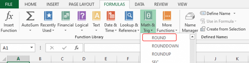
The general Math rules for rounding numbers are followed when using the ROUND in Excel. The function rounds a number either up or down to a specific number of digits based on the number to the right of the rounding digit. The rounding digit is considered as the least significant digit and gets changed depending on the number following it (to the right of it). If the number that follows the rounding digit is from 1 to 4, the rounding digit will remain unchanged or rounded down while numbers 5 to 9 are rounded up by adding 1 digit.

The ROUND formula in Excel is:

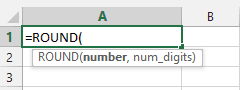
Where:

Number – A required argument that represents the number that has to be rounded. You can use the number itself or a reference cell.

Num_digits – A required argument that represents the number of decimal places you want to show. You can reference the number itself or a reference cell.

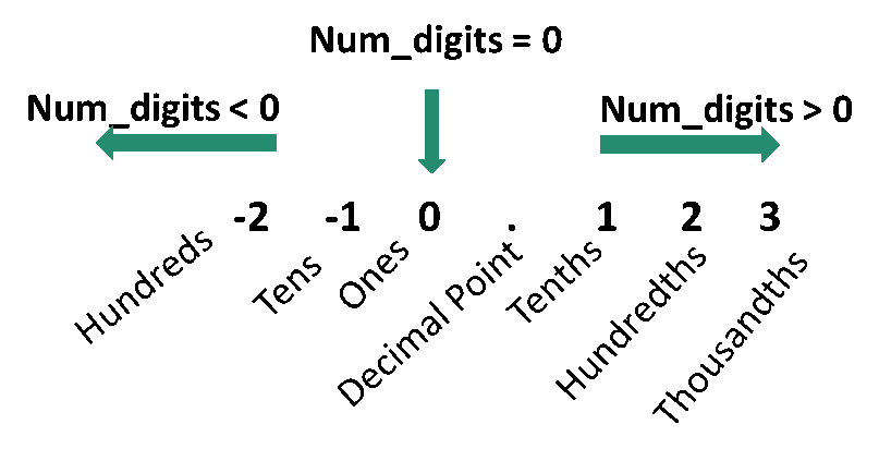
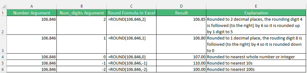
• If the Num_digits is greater than 0 it identifies the number of digits to the RIGHT of the decimal point- tenths, hundredths, thousandths, etc. (See Cells D2 and D3 in the Excel table below)
• If the Num_digits is zero the number is rounded to its nearest integer or whole number. (See cell D4)
• If the Num_digits is less than 0 it identifies the number of digits to the LEFT of the decimal point-ones, tens, hundreds, etc. (See cells D5 and D6)

A graphical presentation of the Num_digits argument in the ROUND formula in Excel:

Consider the following table applying the logic behind the ROUND formula in Excel.

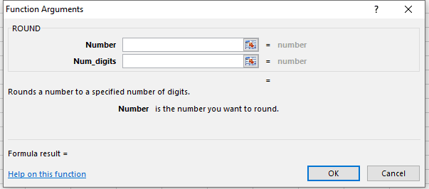
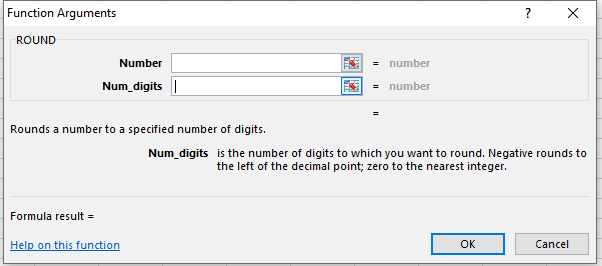
Important TIP: If you need more help with the function after typing the ROUND formula in Excel, use the shortcut CTRL + A (Arguments). An Insert Function Dialog Box with detailed instruction pops up.

Examples on How to Use ROUND in Excel

The ROUND formula in Excel can be combined with other Excel functions and formulas. The Number argument can be used with not only numbers but also cell references, Excel functions, and formulas. You can add, divide, multiply, and apply the SUM, AVERAGE, and IF functions to numbers you’re working with then round the result to the specific Num_digits.

How Do You Use the ROUND function in Excel

How do you use the Round Function in Excel? Assume cost per unit table of 5 products below. If you want to sum all the costs, you can simply use the SUM formula =SUM(B2:B6) which results in $65.258.

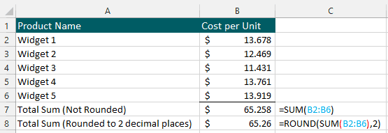
However, if you want to round the total cost of all 5 products to 2 decimal places you can combine the ROUND formula in Excel and SUM formula. The new ROUND formula in Excel will be =ROUND(SUM(B2:B6),2) which gives us a rounded total of $65.26.

Let’s dissect the new ROUND formula in Excel:

1. The Number argument is SUM(B2:B6)
2. This results in the non-rounded total of $65.258 THEN
3. The Num_digits argument of 2, rounds this to the nearest 2 decimal places; S65.26

You can fully utilize the ROUND in Excel by combining it with other Excel functions such as AVERAGE and IF statements to name a few.

How do you Use ROUND Function in Excel Combined with Formulas

Aside from combining ROUND formula in Excel with other functions, using it formulas works as well too. Continuing with the example, assume you want to determine the sales price by adding a 5% markup to each product cost.

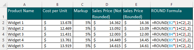
The new ROUND formula in Excel =ROUND(13.678*(1+5%),2) results in a rounded sales price of $14.36.

Let’s dissect the formula for Widget 1 in the following steps:

• The Number argument is $13.678*(1+5%). This adds the 5% markup to the product Widget 1’s $13.678 cost
• This results in a non-rounded sales price of $14.362 THEN
• The Num_digits argument of 2, rounds this to the nearest 2 decimal places. You can also use this depending on the number of decimal places you wish to show.

You are free to use any formula; add, divide, multiply, etc., with the ROUND formula in Excel.

How Do You Use the ROUND Function in Excel for Price Setting

The ROUND in Excel can be used to set prices, ever notice the popular price format that ends with .99? Similarly, You can use the function to round to the nearest .99.

Assume that barriers to entry are low and want your price to be more competitive, you don’t mind minimizing margins to maintain your market share. Using the same sales price we determined before ($14.36), your marketing department suggested a price that ends with .99 can attract new customers and keep existing ones.

How to use the ROUND in Excel in this scenario? By using the ROUND formula in Excel to round the price to its nearest whole number and subtract .01. The new ROUND formula in Excel will be =ROUND(13.678*(1+5%),0)-.01.

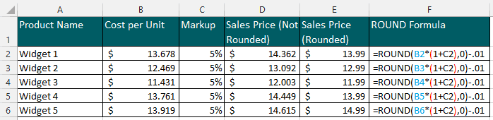
Let’s dissect the formula for Widget 1 in the following steps:

1. The Number argument is $13.678*(1+5%). This adds the 5% markup to the product Widget 1’s $13.678 cost
2. This results in a non-rounded sales price of $14.362 THEN
3. The Num_digits argument of 2, rounds this to the nearest whole number of S14 THEN
4. Subtract .01 from $14.00 gives us a price of $13.99.

Important Points on the ROUND Function in Excel

• The ROUND in Excel rounds numbers 1 to 4 down and rounding the numbers 5 to 9 up.
• To ROUND a number up only, use the ROUNDUP function in Excel.
• To ROUND a number down only, use the ROUNDDOWN function in Excel.
• The ROUND in Excel works with both positive and negative numbers.
• To fully utilize the ROUND formula in Excel you can combine it with other Excel functions and formulas.

Lovenna Tibas Store Manager

Lovenna Tibas is the Store Manager at eFinancialModels, specializing in website management, platform optimization, and customer support. She also writes about financial modeling topics including business valuation and business models, making complex concepts accessible to readers. With expertise in WordPress, Easy Digital Downloads, and e-commerce troubleshooting, Lovenna combines technical skills with a deep understanding of financial principles. Her work focuses on helping businesses leverage digital tools and financial insights to drive growth and make data-driven decisions.

See Full Bio

Excel Financial Modeling General Excel Financial Models