Analyze Financial Data with SUMIF Function In Excel

The SUMIF function is one of the most basic yet widely used functions in Excel. However, as your business grows so does your financial data. To be more successful in business, you need to analyze your financial performance with specific criteria. Simply adding up sales, expenses, and employee hours no longer provides the answer you need to dig deeper into your financials. Enter the SUMIF function in Excel.
To do a little review about the SUM Functions in Excel, here’s a refresher guide on the key fundamentals of SUM functions in Excel.
Excel conditional sum allows you to specify a condition or criterion that must be met first before Excel sums the numbers. It is a function in excel that allows you to do addition based on a condition. Sounds simple enough, right? But there’s more to it, understand it better with step-by-step Excel conditional sum illustrated later below.
How to Use SUMIF Function in Excel? – The Basics
So, how to Use SUMIF Function in Excel? Similar to its more rudimentary peer, SUM function, It is built-in and categorized under Math and Trigonometry function. It is also known as the conditional sum and is used to add cells or numbers based on the single condition or criterion you provide. This criterion can be based on dates, numbers, text, and even cell reference. Aside from logical operators, such as >,<,=, it works with wildcard characters like an asterisk (*).
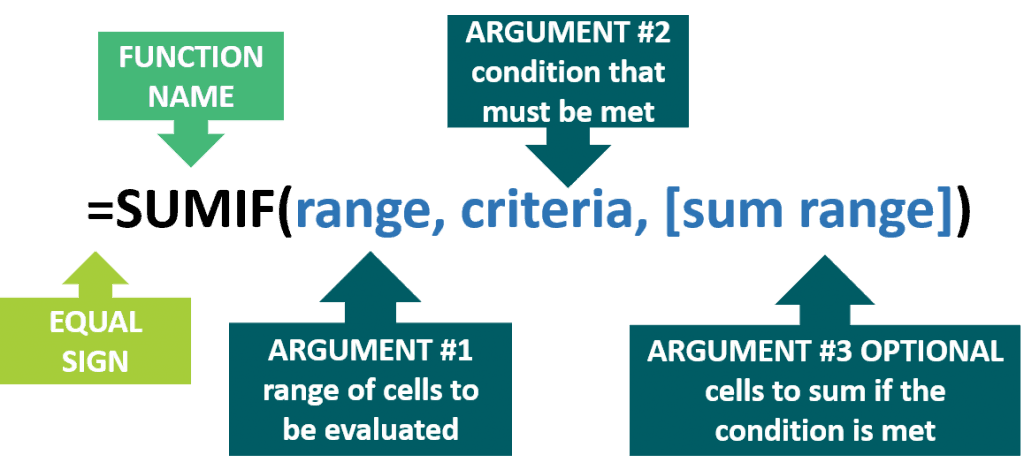
Excel conditional sum has the following arguments:
- Range (Argument#1, required) – Specifies the scope of cells in which the criteria must be applied.
- Criteria (Argument #2, required – The single condition or criterion used to determine which cells will be added. Common SUMIF examples in Excel of a criterion for argument#2 are:
- Any numeric value such as an integer (100 or -100), decimal (.001), date (01/01/2019), time (9:00:00 AM) or logical value (TRUE/FALSE).
- A text string such as “Sales”, “Customer Name”, “Product ID”. The double quotes enable Excel to interpret everything inside as text.
- An expression such as “>100”, “<>0”.
- Sum_range (Argument #3, optional) – is the scope of cells with the numeric values that are to be added if the single condition or criterion is satisfied. Take note this is optional; use it only if you want to add cells other than the
- Range argument (#1). Otherwise, if sum range argument is omitted, values from the Range argument (#1) are added instead.
Examples of Excel Conditional Sum
Comparison Operators (Greater than, Less Than, or Equal to) are widely used in Excel conditional sum.
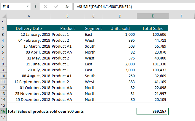
Using Less than
Formula Syntax: =SUMIF(D3:D14,”<500”,E3:E14
Interpretation: Sums the Total Sales in Cells E3:E14 based on units sold in Column D less than 500.
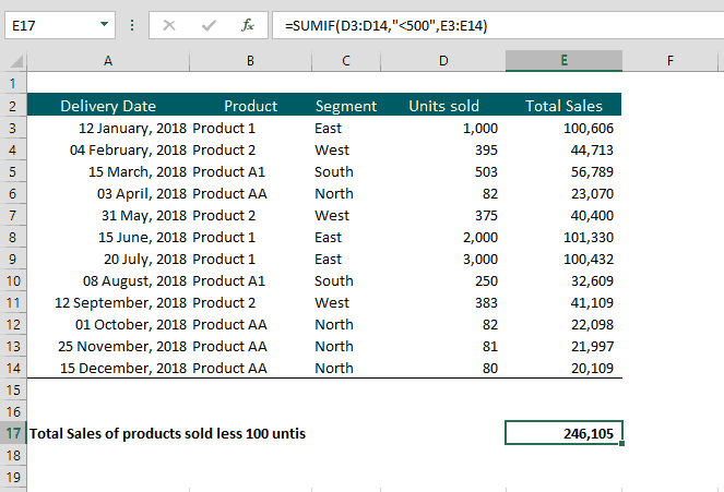
Using Greater than or Equal to
Formula Syntax: =SUMIF(D3:D14,”>=1000”,E3:E14)
Interpretation: Sums the Total Sales in Cells E3:E14 based on units sold in Column D greater than or equal to 1000.
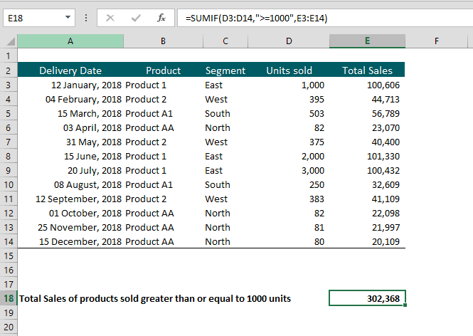
Using Text Criterion
Continuing with our Sales Data Table, you can use the SUMIF function in Excel to identify Total Sales based on the Product Type sold.
Example 1
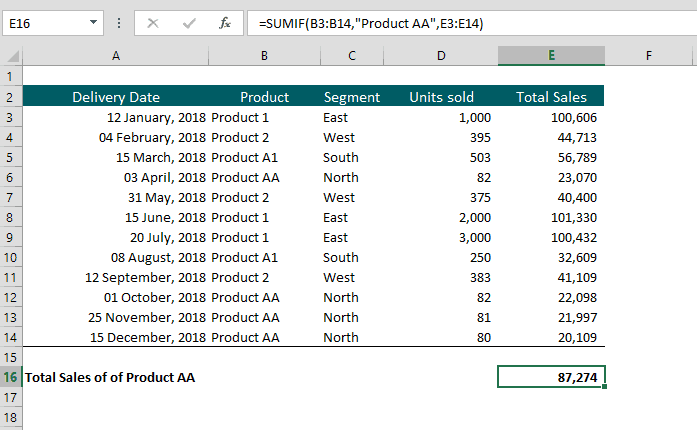
Criterion: SUMIF function in MS Excel based on Text “Product AA”
SUMIF Formula in Excel: =SUMIF(B3:B14,”Product AA”,E3:E14)
Interpretation: Sums the Total Sales in cells (E3:E14) if corresponding Product Type in Column B is Product AA.
Example 2
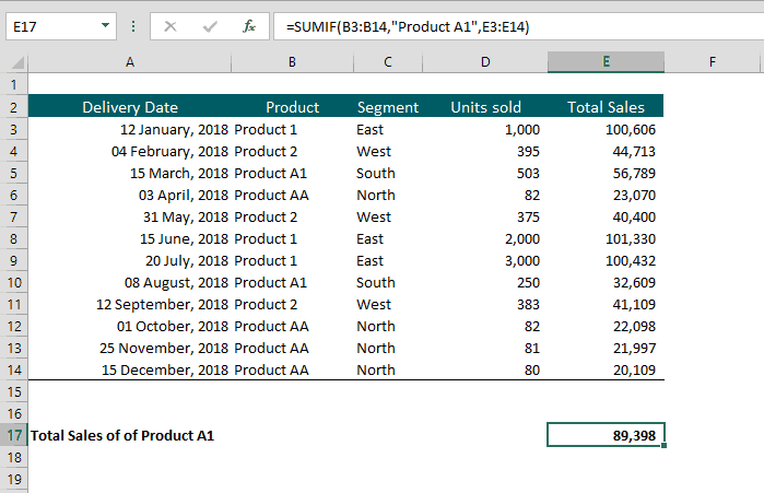
Criterion: Excel conditional sum based on Text “Product AA””
SUMIF Formula in Excel: =SUMIF(B3:B14,”Product A1”,E3:E14)
Interpretation: Sums the Total Sales in cells (E3:E14) if corresponding Product Type in Column B is Product A1.
Example 3
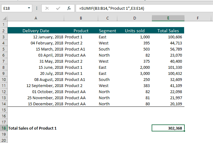
Criterion: Excel conditional sum based on Text “Product 1”
Formula Syntax: =SUMIF(B3:B14,”Product 1”,E3:E14)
Interpretation: Sums the Total Sales in cells (E3:E14) if corresponding Product Type in Column B is Product 1.
Using Cell Reference
Instead of typing a specific criterion, you can use the value of a cell as a reference for your SUMIF formula in Excel. Why use a reference cell? It gives you more flexibility to define your criterion. This is especially useful in financial modeling, where you can present different angles of the same data.
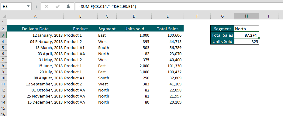
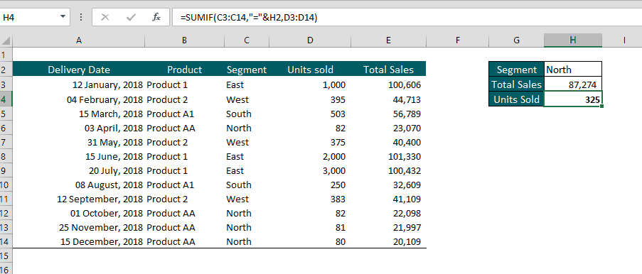
To illustrate, below SUMIF function in MS Excel uses cell H2 as a cell reference for the Segment information needed.
An important thing to remember when you use a logical expression (<,>,=) together with a cell reference is you must use an ampersand (&) in SUMIF formula in Excel to concatenate or link.
Formula Syntax: =SUMIF(C3:C14,”=”&H2,E3:E14) adds the Total Sales based on the Segment you typed in Cell H2 (North). Simply put, the Total Sales to add up are dependent on the Segment input in cell H2. This results at $87,274.
You can use the same SUMIF formula in Excel to get the Units Sold, =SUMIF(C3:C14,”=”&H2,D3:D14).
Using it with Dates
Instead of adding based on text (such as Segment and Product Type) and numbers (Units Sold and Total Sales), you want the criterion to be a date. How to use Excel conditional sum with dates?
You can use Excel conditional sum the same as text and numeric criterion. To illustrate, here are some examples:
Example 1
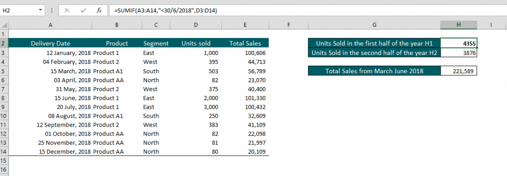
Criterion: SUMIF function in Excel based on less than a given date: Before June 30, 2018
SUMIFFormula in Excel: =SUMIF(A3;A14,”<30/6/2018”,D3:D14)
Interpretation: Sums Units Sold in cells D3:D14 if the corresponding date in Column A is before June 30, 2018.
Example 2
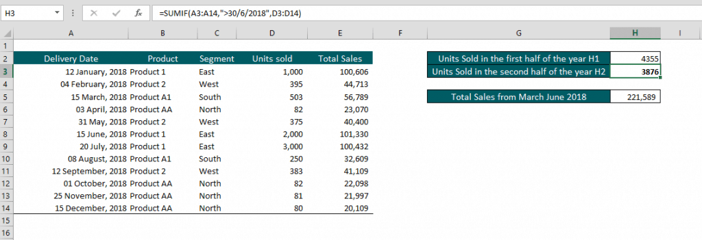
Criterion: SUMIF function in Excel based on greater than a given date: After June 30, 2018
SUMIF Formula in Excel: =SUMIF(A3;A14,”>30/6/2018”,D3:D14)
Interpretation: Sums Units Sold in cells D3:D14 if the corresponding date in Column A) is after June 30, 2018.
Example 3
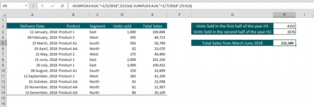
Criterion: Excel conditional sum based on between two dates: March 1 and July 1, 2018
SUMIF Formula in Excel: =SUMIF(A3:A14,”>1/3/2018″,E3:E14)-SUMIF(A3:A14,”>1/7/2018″,E3:E14)
Interpretation: Sums Units Sold in cells D3:D14 if the corresponding date in Column A is between March and July 2018.
Using a WILDCARD Reference
Wildcards are special characters that can take the place of any character in a text criterion and is useful when you need to find partial matches. Excel Wildcard Characters are:
- An asterisk ( * ) represents a series of characters in your text criterion for a SUMIF function in Excel (one or more characters).
- Question mark ( ? ) represents a single character in your text criteria for a SUMIF function in Excel (any one character).
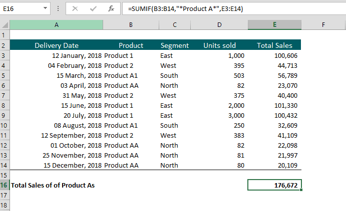
For example, based on the Sales Data Table, you have two product types of Product A, Product AA, and Product A1. Assume you want to sum up Total Sales based on all Product As. To solve this, use SUMIF formula in Excel =SUMIF(B3:B14,”*A*”,E3:E14). Note that SUMIF function in Excel is not case-sensitive, the SUMIF formula in Excel =SUMIF(B3:B14,”*a*”,E3:E14) will have the same result.
Chief Points to Remember About Excel Conditional Sum
It is one of the vital tools to have in your arsenal of MS Excel functions; below are some main points to remember when using it.
- Excel conditional sum can be applied to a single column criterion and a one-column criterion only. For multiple criteria, use the other SUMIFS function in excel.
- The Range and Sum_range criterion in Excel conditional sum should be in ranges. For example, a Formula Syntax of =SUMIF(D3, D10, D14,”>500”, E3:E14) will not work.
- Numerical values in your criterion parameter do not have to be enclosed with double quotation marks.
- Logic expressions and text such as “>=1000”, “<=10”, “=100”,” Product AA” etc. have to be enclosed in double quotation marks.
- #VALUE! Error happens when the criterion parameter is a text string that is more than 255 characters long. To fix this, you can break down or shorten it by using a concatenate function, the Ampersand (&). For example, the Formula Syntax =SUMIF(B3:B14,”lengthy text”&” another lengthy text”, E3:E14).
- Excel conditional sum in Google sheets is the same with MS Excel. So, there is not a lot of adjustments needed to for using the sheet’s SUMIF function.

