5 Steps on How to Use VLOOKUP Function in Excel

Microsoft Excel boasts a wide number of lookup and reference function but no other is commonly known than the VLOOKUP function in Excel. If you’re working with tables most of the time, from multi-year financial statements to inventory systems, understanding how to use VLOOKUP function in Microsoft Excel can come in very handy. However, for beginners, the Excel VLOOKUP function can be intimidating to wrap their heads around.

In this article, we will discuss what the Microsoft Excel VLOOKUP function is and the 4 arguments in the Excel VLOOKUP formula. We will also illustrate common Excel Spreadsheet VLOOKUP examples in Excel that highlight why users gravitate to it and the common errors and limitations encountered.

What the Letter “V” Stands for in Excel VLOOKUP Function

Excel Spreadsheet VLOOKUP function is one of the most widely used Lookup & Reference Functions. The “V” in the VLOOKUP function in Excel stands for vertical representing the vertical lookup it performs. It always looks up a value in the leftmost column of a table and the function returns a corresponding value from the column to the right.

If the Excel Spreadsheet VLOOKUP formula does not find an exact or approximate match, it will return the #NA error.

The Excel VLOOKUP formula

Where:

Lookup_Value
– The value to find which can be numeric values, cell references, or text strings. For the Excel VLOOKUP formula to work properly, the Lookup_value must be at the left-most column of the array (Required argument).

Table_Array
– The cell ranges where the Excel VLOOKUP function will search from. (Required argument).

Col_Index_Num
– Represents the column numbers within the table_array to retrieve the data or return value needed (Required argument).
– A Col_Index_Num of 1 instructs the Excel VLOOKUP formula to get the value in the 1^st column.
– A Col_Index_Num of 2 instructs the Excel VLOOKUP formula to get the value in the 2^nd column.

[Range_Lookup]
– Also known as the fourth argument, it defines whether the Excel VLOOKUP function searches for an exact match or approximate match of the lookup_value (Optional argument).
– When the range lookup is FALSE, it will give you an exact match.
– When the range lookup is TRUE, it will give you an approximate match, this is the default and you can simply omit it.

5 Steps on How to Use VLOOKUP function in Excel

Step 1. Arrange Data Suitable for VLOOKUP function in Excel

Excel VLOOKUP function works from left to right so the first step in successfully using the function is to arrange the data wherein the value you want to search is to the left and the corresponding information needed to retrieve is on the right.

Step 2. Identify the 1^st required argument; the Lookup_Value

This step instructs Excel on what to look for. VLOOKUP function in Excel can look up numbers, dates, names, and even wildcard characters.

Step 3. Define 2^nd required argument, the Table_Array

The 2^nd required argument directs the Excel VLOOKUP formula where to find the Lookup_Value and the required return value by selecting the cell ranges, named range, or table. The array can be on the same worksheet, a separate sheet in the same workbook, or a completely different workbook.

Step 4. Specify Column Numbers, Col_Index_Num, from the Table_array

This step inputs the last of the 3 required arguments and specifies which column to get the required return value. Excel uses the column number (not the column letter) and is relative to the range of cells selected. Keep in mind the Col Index number is user-defined, the Excel VLOOKUP formula by itself cannot locate the column number.

Step 5. Choose between Exact (FALSE) or Approximate Match (TRUE)

This 5^th step is optional and instructs Excel to find an exact or approximate match of the Lookup_value argument. Even if it’s optional, this argument is essential as selecting the wrong type will lead to different results. Omitting the match type has the same effect as selecting TRUE for an approximate match.

To illustrate the 5 steps, we will use the list of countries and their respective economic data below.

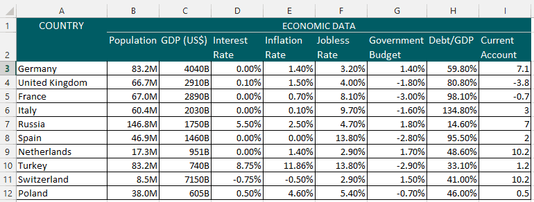
Using the VLOOKUP function in Excel, lookup the interest rate for Switzerland.

1. The lookup table has been arranged so that the data can be used for the VLOOKUP function in Excel. The value to lookup is located on the left-most column, the list of countries, and the return value, in the form of economic data of each respective country,  is to the right.
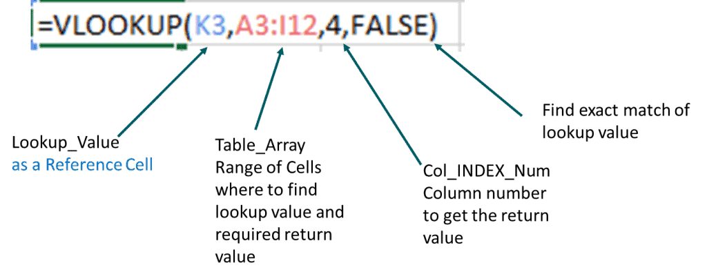
2. The Lookup_value is found on the left-most column in the table. For this example, it is”Switzerland”
3. The Table_Array is the range of cells where to find the return value needed, range A3 to I12.
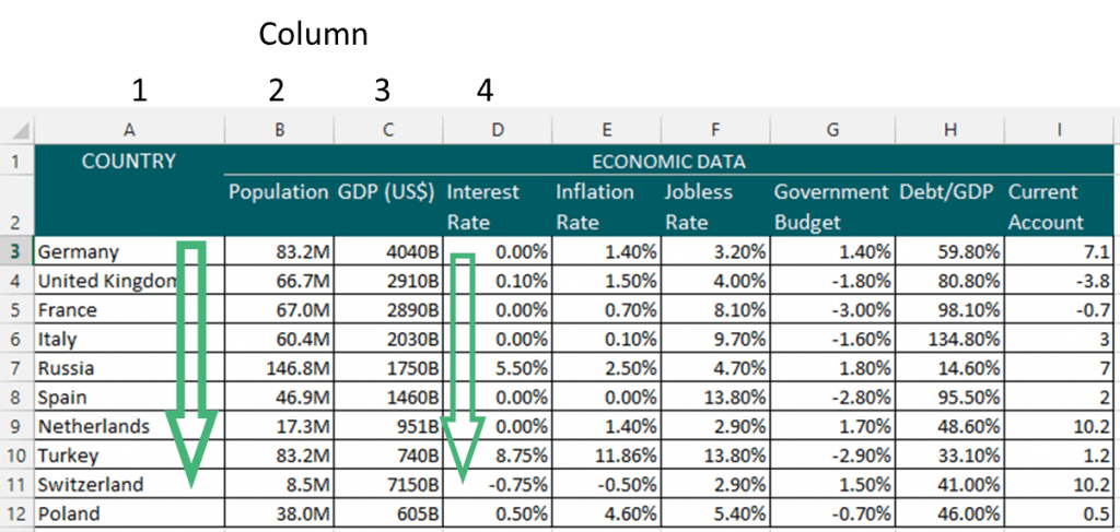
4. By looking at the Table_Array, we can pick out the Interest Rate column in the 4^th column from the left. So, the Col_Index_Num is number 4.
5. Since we are searching for the exact match of Switzerland’s interest rate, we select FALSE.

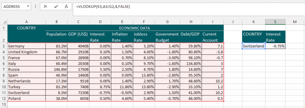
Following the 5 steps, we come up with the Excel VLOOKUP formula below which gives us the interest rate of -0.75%.

The Excel Sheet VLOOKUP formula searches vertically in the left-most column. When it finds the exact match for the Lookup_Value, Switzerland, it then looks to the right towards the 4^th column (as indicated by the Col_Index_Num argument). The VLOOKUP function in Excel gets the return value of -0.75%.

Different Ways How to Use VLOOKUP Function in Excel

Dynamic 1-Way VLOOKUP Example in Excel

The previous VLOOKUP Example In Excel uses a hard-coded Lookup_Value so the return value will always refer to the country Switzerland. What if the interest rate for another country is needed?  How to use VLOOKUP function in Excel in this scenario?

You can input another country name directly into the formula but this is prone to errors. How to use VLOOKUP function in Excel for a dynamic lookup? By using a cell reference as the Lookup_Value.

The Excel VLOOKUP formula below replaces the hard-coded Lookup_Value “Switzerland” with reference cell K3. Whatever country name is entered in the reference cell will always be the Lookup_Value.

When the Lookup_Value is a text string, the Excel VLOOKUP formula can be used with wildcard characters (*) and (?).

In the below example, the 2 asterisk characters “*”&K3&”*” indicates that anything in between should be matched and return the corresponding result.

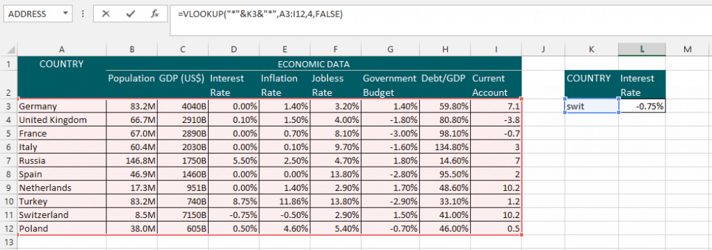
Another way to make a dynamic lookup is to create a drop-down list. Using the drop-down list, users can easily select the country name and quickly avoid any invalid input.

Dynamic 2-Way VLOOKUP Example in Excel

VLOOKUP function in Excel just like any other Excel function can be combined with another function to create a more versatile search.

From the previous examples, for the Excel VLOOKUP formula to perform properly the column number must be given. The VLOOKUP function in Excel without the Col_Index_Num will return an error.

Continuing with our example, assume you want to use the VLOOKUP function in Excel to return the interest rate for Switzerland. However, the Col_Index_Num argument is not given or unknown.

To perform a dynamic 2-way lookup, we must combine Excel VLOOKUP formula with the MATCH formula. The MATCH function will provide the column number for the Col_Index_Num argument. The MATCH function returns the relative position of data within a range of cells. The position is the intersection of a row and a column and is in the form of a number.

The combined VLOOKUP function in Excel and MATCH function performs a 2-way lookup.

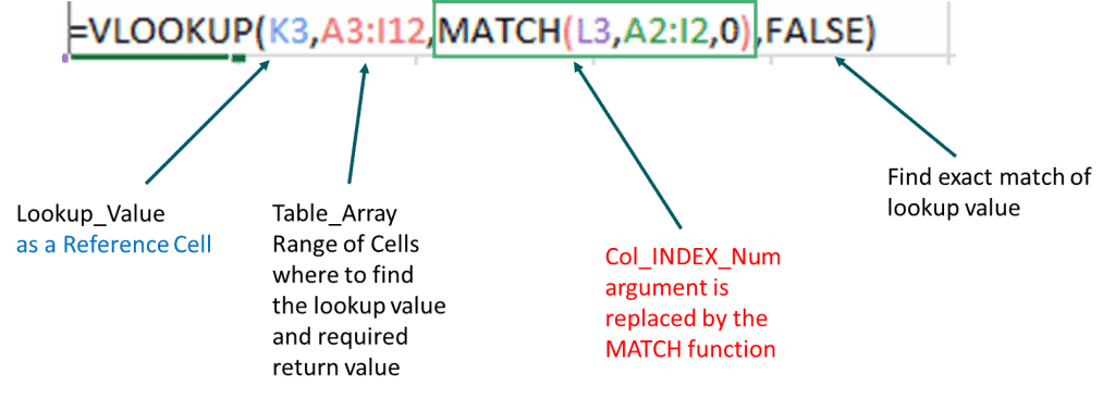
By combing the VLOOKUP function in Excel and MATCH function a more dynamic search is performed. Simply input any country name from the list and return value can be any economic data preferred.

Without changing anything in the Excel VLOOKUP formula, simply input another preferred country and economic data. In the below example, Italy’s Jobless Rate is 9.70%.

Multiple Criteria VLOOKUP using the Helper Column

Another way to use the VLOOKUP is to use look through multiple criteria, but given the VLOOKUP formula’s limitations, we will need to use what is called the helper column. So given this example:

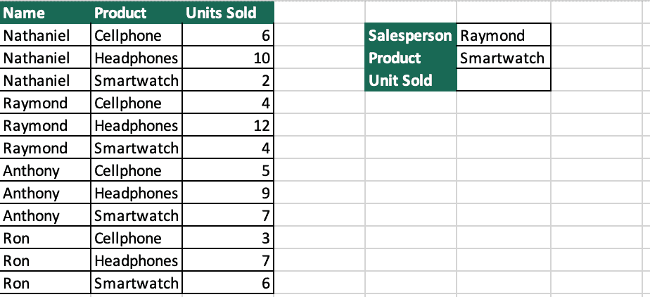
If we want to get the results of how many smartwatches Raymond sold, we cannot just use VLOOKUP because it will only return the first result based on the specified lookup value. To work around that, we need what we call a helper column. To do a Helper column, we need to first insert a column (Column A) on the left-most part of the table, then combine the entries of the two lookup columns using this Formula:

= B2&” “&C2

We then just drag it down until the last row. Then, we can use VLOOKUP in cell G4:
=VLOOKUP(G2&” “&G3,A2:D13,4, FALSE)

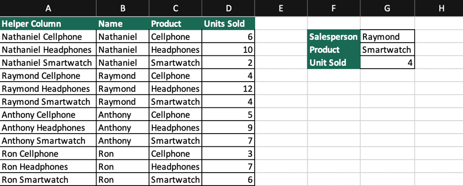
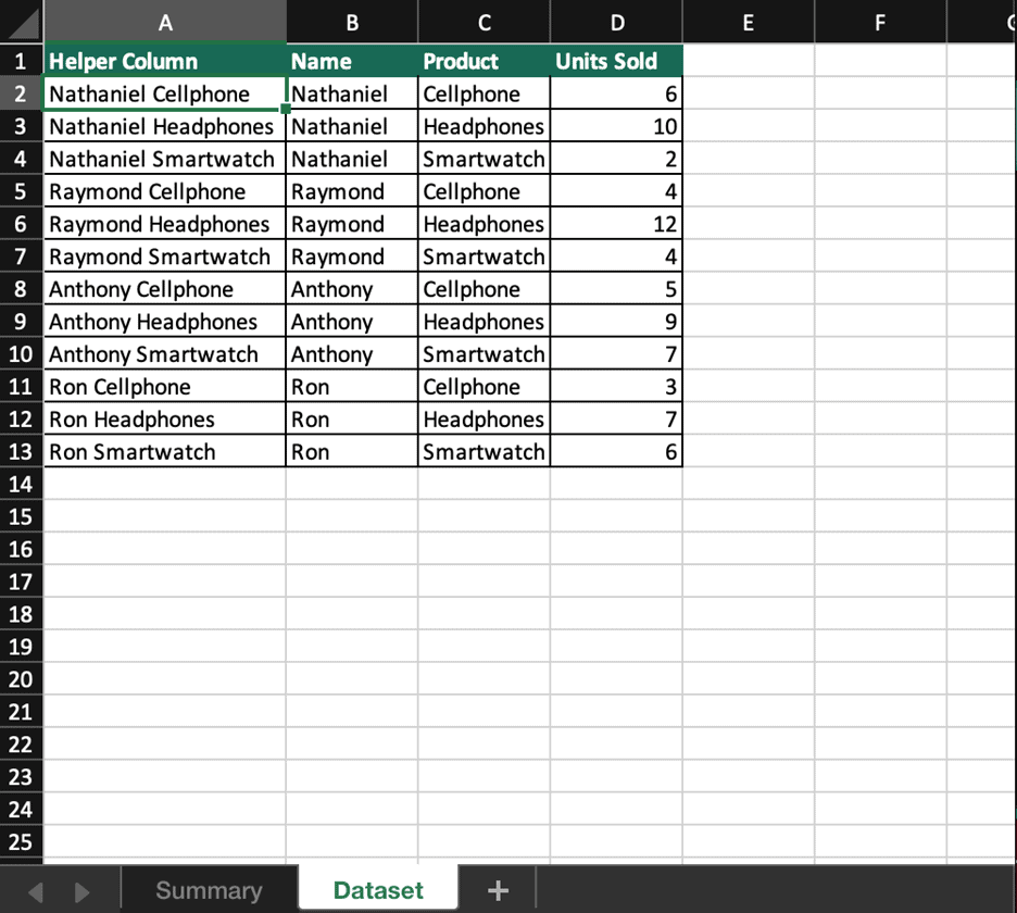
Now, we are able to lookup two different criteria’s and looked up the value we need through the use of a helper column.

How to Use VLOOKUP Excel from sheet to sheet?

When we use this command, we usually don’t have the data place the lookup beside or within the datasheet, we usually do excel VLOOKUP in another sheet. We do  VLOOKUP Excel in separate sheets because we usually use Vlookup to make it convenient and easy to look for data in the dataset or spreadsheet.

So, how to use VLOOKUP from sheet to sheet? To make thing convenient, I’ll use the previous example:

Now, this is our current dataset, we put it in on a separate sheet as it is normally the case. Next, we want to know how many cellphones Raymond has sold so:

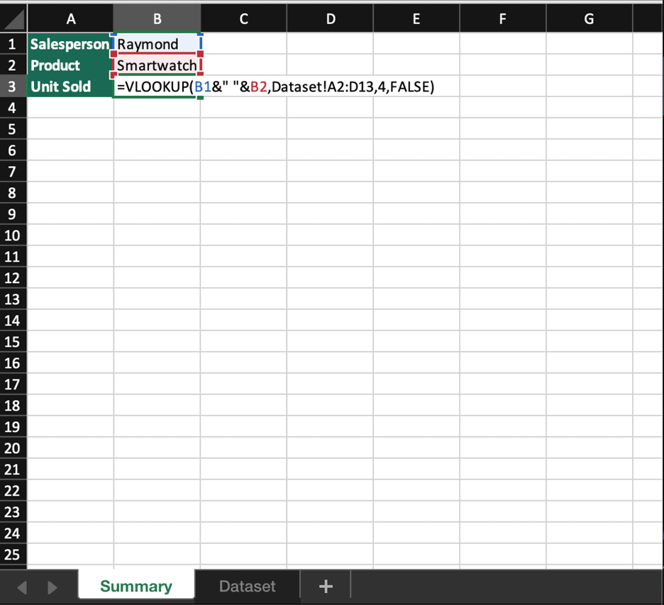
Using the previous example, we can see that for the table array, we added the “Dataset!” in front to indicate that we are pulling this from another sheet with that name. Using Vlookup in multiple sheets follow the same principle. We just add the name of the sheet in front of the table array, and add an exclamation point in between.

 Possible Reasons Excel VLOOKUP Function is Not Working

The VLOOKUP function in Excel is widely used and a popular Lookup & reference function but it is not without limitations. Not understanding these limitations can lead to errors.

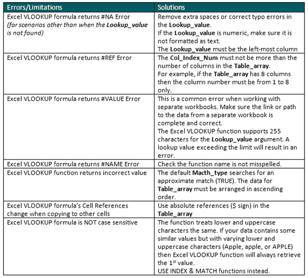
Caveats When using Excel VLOOKUP Function

• The VLOOKUP function in Excel always looks to the right. The function searches the left-most column and returns the value from the right column. When you need to lookup value within a row and the data is arranged horizontally, then use the HLOOKUP function. If a more flexible search is needed such as the ability to look up, down, right, or left, then use the INDEX MATCH combination.
• Excel VLOOKUP formula is NOT case sensitive so your data must not have duplicates. When the lookup value is a text string, the function works using wildcard characters.
• Although the [Range_Lookup] is the last and optional argument, it plays an important role in the results. Incorrectly selecting TRUE/FALSE will yield different results.

Lovenna Tibas Store Manager

Lovenna Tibas is the Store Manager at eFinancialModels, specializing in website management, platform optimization, and customer support. She also writes about financial modeling topics including business valuation and business models, making complex concepts accessible to readers. With expertise in WordPress, Easy Digital Downloads, and e-commerce troubleshooting, Lovenna combines technical skills with a deep understanding of financial principles. Her work focuses on helping businesses leverage digital tools and financial insights to drive growth and make data-driven decisions.

See Full Bio

Excel Financial Modeling General Excel Financial Models