What is the Match Function in Excel?

What is the Match Function in Excel? The official headquarters of the Prime Minister of the UK is at 10 Downing Street. The official residence of the President of the USA is at 1600 Pennsylvania Avenue. The famous detective of all time Sherlock Holmes resides in 221B Baker Street. Last but not least, the most lovable yellow sea sponge SpongeBob SquarePants lives in 124 Conch Street.

Of the hundreds of interesting locations (real or fictional) across the world, without its exact address or the street number, no one will know about these places and will be left in obscurity.

Similarly in financial analysis when working with large data, lookup and reference functions such as cross-referencing different data sets, providing information about a range of cells, and looking up values are essential. Another important lookup function is the Excel MATCH function.

The MATCH function in excel locates the relative position of the value from the range of cells. In this article, we will discuss what is an Excel MATCH function and how the MATCH formula in Excel spots the value’s position. We will also learn how to use the function by illustrating examples.

How To Use the MATCH Function in Excel:

Understanding The Location Tool With Excel MATCH Function

How to use the MATCH Function in Excel? The MATCH function in Excel is one of the Lookup and Reference functions and is used to look for the position of a number, text, date, name, etc. within a range of cells. So whether if you are looking for a dollar amount, customer name, product ID, or delivery date in your spreadsheet, Excel MATCH function will always return the position in a form of a row number or column number it is located.

The MATCH formula in Excel Sheet:

Where:

Lookup_value
– Represents the value to find which can be numeric, text string, cell reference, or logical value. This is a required argument.

Lookup_array
– Represents the range of cells to search from and is the 2^nd required argument in the formula.
– The MATCH formula in the Excel sheet cannot search for multiple ranges of cells. In other words, the MATCH function in Excel can only search in one direction.

[Match_type]
– Defines whether to return an exact match or the closest match. This is an optional argument.
– This can be set to 1, 0, or -1. Follow the below table of instructions to help you define the argument.

To learn how to use the MATCH Function in Excel, please feel free to check out our video here:

MATCH function in Excel Examples:

Excel MATCH function is simple and easy to use, here are Match Function in Excel examples to help you. Assume below a table of Auto and Truck Manufacturers and their respective market cap.

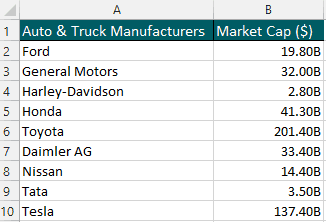
Using the MATCH formula in Excel Sheet we can search the relative position of the exact and approximate match of the manufacturer name and market cap.

Excel MATCH Formula for Exact Match

Searching for the relative position of a value’s exact match is widely used compared to the other match types.

For example, where is General Motors company located on the list?

The MATCH formula in Excel Sheet=MATCH(E2,A2:A10,0) returns the number 2.

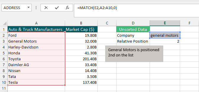
A breakdown of the MATCH function in Excel is as follows:

Lookup_value	Lookup_array	[Match_type]
Value to find	Where to find the value	Exact Match
Cell E2	A2:A10	0

When the Lookup_value is a text string, the Excel MATCH function is not case sensitive. Wildcard characters like the question mark (?) and asterisk (*) can also be used.

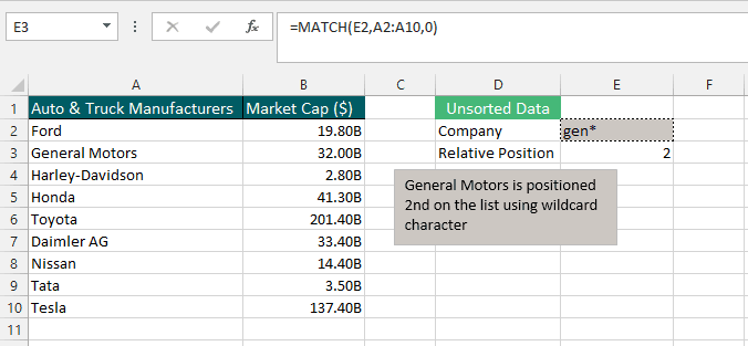
Excel MATCH Formula for Approximate Match

Although the MATCH function in Excel is commonly used for exact matches, sometimes an exact match is not possible. Searching for the closest or nearest match is still possible based on the [Match_type] argument given.

One important element to understand when searching for the closest or nearest match is the data must be sorted, so the Lookup_Array must be in ascending or descending order.

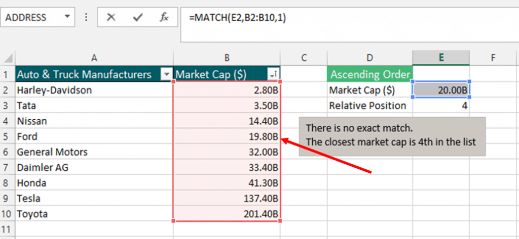
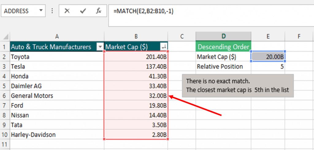
For example, assume you want to search if a market cap of $20B is in the list.

If the data is sorted in ascending order (from smallest to largest, 0 to 9, or A to Z), the MATCH function in Excel searches the closest or nearest match that less than (below) the Lookup_value.

The MATCH formula in Excel Sheet =MATCH(E2, B2:B10,1) results in 4. The market $19.80B is the 4^th market cap on the list and is the closest lower approximate of $20B.

On the other hand, if data is sorted in descending order (from largest to smallest, 9 to 0, or Z to A), the MATCH function in Excel searches the closest or nearest match that more than (above) the Lookup_value.

The MATCH formula in Excel Sheet =MATCH(E2, B2:B10,-1) results in 5. The market cap of $32B is the 5^th market cap on the list and is the closest higher approximate of $20B.

Important Notes using Excel MATCH Function

• The MATCH function in Excel returns the relative position of a cell containing the information we are searching for and not the information itself.
• Excel MATCH function when dealing with text values is not case sensitive. The Lookup_value can be in lowercase, uppercase, and wildcard characters.
• The MATCH formula in Excel Sheet returns the first position of the Lookup_value if the Lookup_array argument contains more than one occurrences of the Lookup_value.
• Excel MATCH formula returns the #N/A error if the Lookup_array does not find the exact match.
• MATCH function in Excel can be combined with other Excel functions but it is usually used as INDEX and MATCH functions.