The COUNTIF function in Excel counts the number of cells that meet a single condition. This formula is a powerful tool, especially in financial modeling, which gives you the ability to quickly check the contents of a large data table by category. The formula offers more than just simple conditions for counting numbers, text, value, and blank cells. Learning how to use COUNTIF function Excel allows you to improve the readability and understanding of the data tables in Excel.

The COUNTIF examples in Excel mentioned in this article will help you how to count data from a table that meets certain conditions such as “less than“ or “more than”.

The Nuts And Bolts of the COUNTIF Formula

The COUNTIF function in Excel is a built-in function that is available under the statistical function menu in Excel. At its core, it is very similar to the COUNT function in Excel as it counts the number of cells. The difference between COUNT and the COUNTIF function is that COUNTIF only includes the number of cells that meet certain criteria. This allows a more granular analysis of your spreadsheet data.

See also the difference between the five ways to count in Excel: How to Use Count Functions in Excel for Business.

The COUNTIF Formula in Excel

The formula is structured in a way so that only two elements are required: Where to search and for what.

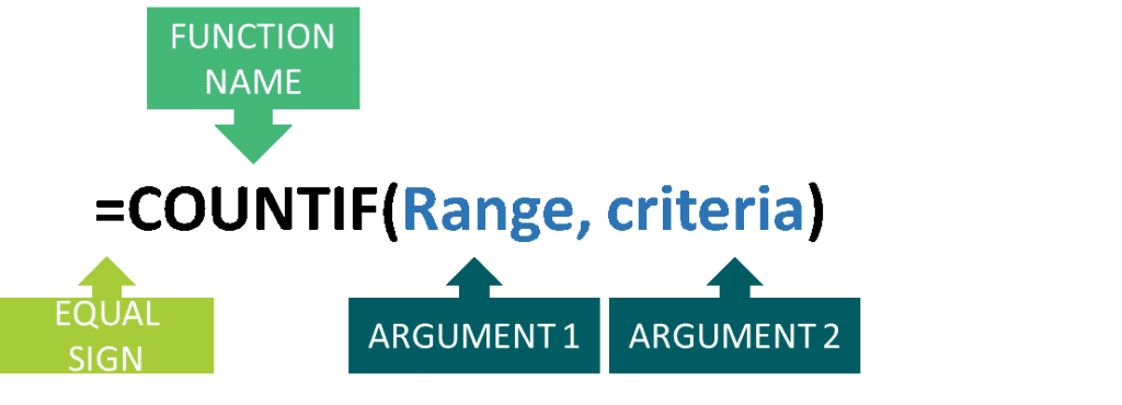
The COUNTIF function requires two arguments:

• Range: The range of cells that will be counted provided the cell contents meet the criteria. The criteria must be satisfied in order to be counted. Otherwise, the cell will be ignored.
• Criteria: This defines which cells to count. The function will only count cells that meet this criterion.

Some examples on which criteria can be used:

1. Numbers (5,100,.10.2.5)
2. Dates and Time (10:00,29/01/2018)
3. Text (“Mr Smith”,”January”)
4. Logical Operators (<,>,<>,=)
5. Wildcard characters (*,?)

For more information, please refer to Microsoft’s Website.

A criterion using No. 1 to 4 in the COUNTIF function in Excel can be used as a direct or exact match with the single criteria whereas using No.5, the question mark or asterisk can be used as a partial match.

As you can see, different variations and possibilities turn this function into a powerful tool to extract and analyze data in financial modeling. Let’s look at some examples now.

COUNTIF Example In Excel No. 1: Numbers & Text

This is one of the most basic uses of the COUNTIF function in Excel. You can use the COUNTIF function in Excel to count the number of cells where a specific text is contained.

For example, using a Sales data list below we count the number of cells containing a sales person’s name.

The COUNTIF formula for Excel =COUNTIF(C3:C18, ”John”) gives us a total count of 5. The Range is represented by cell range (C3:C18) and Criteria is the text (name) “John”.

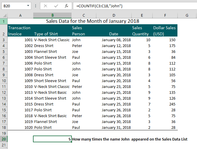
It is important to keep in mind that a Text criterion is NOT case sensitive so if you type “john” or “JOHN”, this will not change the result.

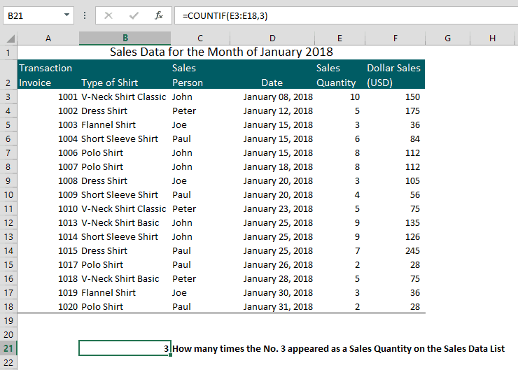
How to use the COUNTIF function in Excel for a Number criteria? It is basically the same. Assume we want to count the number of cells containing the number 3 under Sales Quantity (Column E).

The COUNTIF formula for Excel =COUNTIF(E3:E18,3) results in a total count of 3. The Range is represented by cell range (E3:E18) and Criteria is the number 3.

Example No. 2: Wildcard Characters

In working with large data, it is unavoidable to have your Text criteria in several forms or variations.

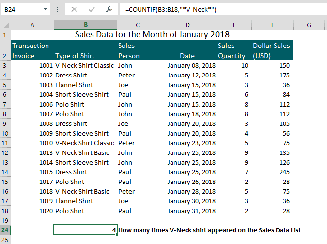
Notice under Type of Shirt (Column B), a V-Neck shirt sold in the retail store has two versions – Classic and Basic. Assume, we want to count the number of cells that contain the text “V-Neck shirt” only and ignore the texts “Basic” and “Classic” in the Sales Data List.

Using the COUNTIF function in Excel, you can combine wildcard characters to filter the results.

Wildcard characters are special characters representing one or more other characters. The asterisk (*) is the most common and is used to match zero or more characters of characters.

• Asterisk (*) – matches any one or more characters. This is used when counting cells containing a specific word or a character(s). In summary, we can also say that a question mark matches any single character.
• Question mark (?) – matches any single character. This is used when counting cells beginning and/or ending with certain characters. In summary, we can also say that an asterisk matches any sequence of characters.

The COUNTIF formula for Excel =COUNTIF(B3:B18,”*V-Neck*”) results in a total count of 4. The Range is represented by cell range (B3:B18) and the Criteria is the “V-Neck”.

Example No. 3: Greater Than, Less Than, Or Equal To

COUNTIF function in Excel works also on counting the number of cells using logical operators (<,>,<>,=). Understanding how to use COUNTIF function Excel can help you count cells with values greater than, less than, or equal to, etc.

Based on the Sales List, you can analyze your sales performance based on Dollar Sales for the month similar to below.

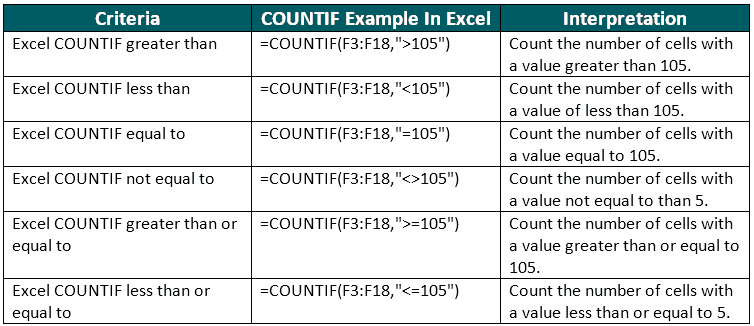
Because we used these excel functions, we’re able to conveniently count how, let’s say, many times dollar sales reached greater than or equal zero to USD 105.00.

Therefore, we can say that COUNTIF function in Excel- can help analyze your business’ performance and compare it with key metrics to give you insights.

Example No. 4: Dates

If you have a similar list like our sales data example where transaction dates are important, you can use the COUNTIF function in Excel to count the number of cells that match a specific date.

You can also use the COUNTIF function in Excel to count the number of cells that match a range of specific dates, you can use the logical operators greater than or less than a specific date.

Example No. 5: Cell Reference

Instead of typing the Text, Number, or Date criteria within the formula, you can use a reference cell. This will allow you to be more versatile, you can change your criteria without having to change the formula itself which will also help you avoid any errors. For example, people usually use cell a1 as a reference cell where you put your searches for the COUNTIF function in Excel.

How to use COUNTIF function Excel to count text and numbers using cell references? To illustrate, let’s incorporate this in our prior COUNTIF examples In Excel.

COUNTIF(C3:C18,B20) uses cell B20 as the reference cell. Whatever text or number is entered in Cell B20 will be the criterion.

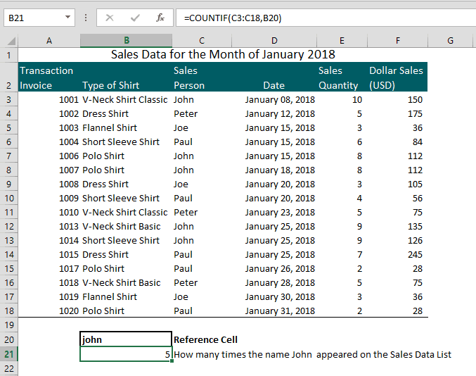
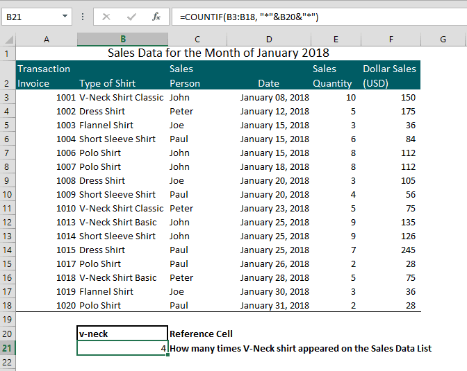
How to use COUNTIF function Excel using wildcards with cell references? By simply linking the cell reference with your COUNTIF formula using a concatenation operator- the ampersand (&).

In our No.2 COUNTIF example In Excel, instead of typing “*V-Neck*”” directly within the formula, you can type it in your reference cell, B20. Your new COUNTIF formula for Excel will be =COUNTIF(B3:B18, “*”&B20&”*”)

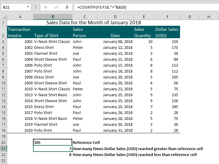
How can Excel count cells that are greater than or less than a certain condition using a cell reference?

By enclosing the logical operators in quotes (“ “)  and adding an ampersand (&) before your selected reference cell (recall the symbol & will serve as linking operator).

Using COUNTIF example In Excel No. 3 and Cell B20 as your reference cell, the new COUNTIF formula for Excel will be =COUNTIF(F3:F18,”>”&B20) formula. This gives us a total count of 7.

Common Issues with the COUNTIF Function in Excel

If you followed the examples and tried the formula with your own business data but were not able to get it to work, take a look at some of the most common issues. related to this function:

• #NAME? error: Double-check the range of cells, criteria, cell references, use of ampersand, double quotes, and spaces. At times you may find the error was caused simply by a misspelling.
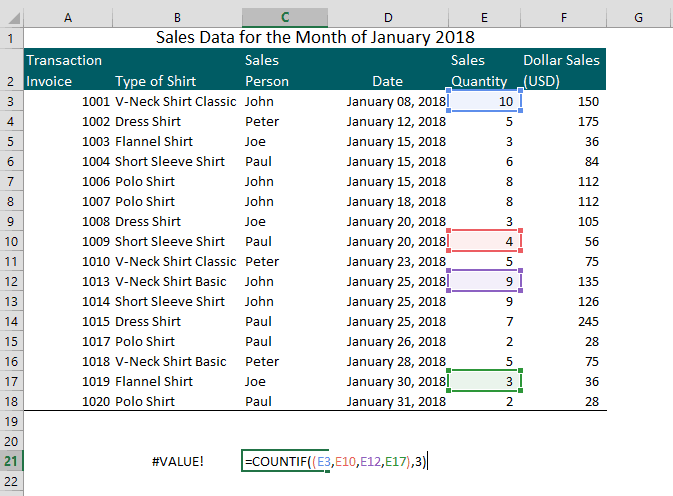
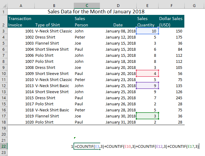
• Non-contiguous (not adjoining) range of cells: In our COUNTIF example in Excel No. 1, the formula =COUNTIF(E3:E18,3) uses E3:E18 cell range to count the cells containing number 3. But what if you only want specific individual cells to be counted, say E3, E10, E12, and E17? The result is a #VALUE! Error. The COUNTIF function in Excel does not work if the cell ranges are not adjoining nor does the function allow you to specify several individual cells.

• To fix this, you can use a combination of several COUNTIF functions to count in Excel.

• Color formatted cells: Unfortunately, the COUNTIF function in Excel does not allow using color formats as a criterion.
• Ampersand (&) and quotes (“ ‘”): This may be confusing and tricky at first but identifying what you are matching with your criteria is the key to understanding how to use COUNTIF function Excel with an ampersand (&) and quotes (“ ‘”)
  • If you use a number or a cell reference in the direct or exact match criteria, you do not need to use both ampersand and quotes.
  • If a criterion includes text, wildcard character, or logical operator with a number, you must enclose it in quotes.
  • If a criterion is with a cell reference or another Excel function, you must use both ampersands to concatenate and quotes.
• Counting non-blank cells – To use COUNTIF Excel for non-blank cells, we need to use the COUNTA Function. The COUNTA function counts all cells containing values, texts, logical values, and errors. It leaves out blank cells.
• Multiple Criteria: When you intend to count multiple criteria, please use the COUNTIFS formula in Excel instead.