
0 ITEMS

How to Make Smart Decisions with 6 Key Financial Metrics?
Table of Content
- Our Concept of Key Financial Metrics at eFinancialModels
- Benefits of Using Key Financial Metrics
- Key Financial Metrics to Make Solid Investment Decisions
- How to Know When to Use Which Key Financial Metric

Understanding key financial metrics is essential for making informed investment and business decisions.
- Metrics like NPV, IRR, and payback period help evaluate the profitability and risk of projects.
- Cash yield and cash on cash multiple focus on actual cash returns, useful for buy-and-hold strategies.
- Combining different metrics provides a clearer picture of long-term value and investment potential.
- Each metric has unique advantages and limitations, so knowing when and why to use them improves decision quality.
- Using these metrics with financial models ensures smarter planning and better strategic choices.
This article guides you through the most important financial metrics to support strong business and investment decisions.
Our Concept of Key Financial Metrics at eFinancialModels
Key financial metrics are quantifiable measures used to evaluate the expected financial performance of a business or investment. These metrics help analysts, investors, and management assess a company’s financial health and profitability. The purpose of financial metrics is to provide insight into the financial performance of an asset, business, or project. By analyzing these metrics, stakeholders can make informed decisions about budgeting, business strategy, and investments.
Often, financial metrics are assumed to be the same as financial ratios. Both quantitative measures provide insight into a company’s financial health and performance. However, there are some critical differences between the two. Financial ratios are specific calculations that compare two or more economic variables. For example, the debt-to-equity ratio compares a company’s debt to its equity. They can also be used to compare companies in the same industry. Financial metrics, on the other hand, may be calculated as a ratio or a simple computation, such as revenue or net income. Financial metrics provide insight into how well a company performs but do not necessarily compare one variable to another.
At eFinanciallModels, we broadly categorized business metrics into financial ratios, key performance indicators (KPIs), and financial metrics. Here, we will discuss a glimpse of the first two categories and explain how the third can help you make solid investment decisions.

Financial Ratios
Financial Ratios are relationships between two or more financial figures used to analyze, better read, and compare a company’s financial performance and situation. They are mainly geared towards better reading and comparing financial statements. Financial ratio assumptions can also be used for budgeting.
Financial ratio analysis is an impartial technique to determine a company’s success. While it cannot account for unforeseen or extraordinary events, it does offer a mechanism for businesses to swiftly understand crucial information and make decisions based on facts rather than feelings or bias. Examples of key financial ratios include:
- Bank ratios
- Efficiency ratios
- Liquidity ratios
- Profitability ratios
- Valuation ratios
Key Performance Indicators (KPIs)
A Key Performance Indicator (KPI) is a business metric that measures a company’s performance relative to its goals and objectives. It is used to track progress over time and identify areas for improvement. KPIs are used primarily to improve a company’s operating performance daily by following the relevant business metrics.
In the context of financial metrics, KPIs can be defined as specific financial indicators measuring the effectiveness of an organization’s financial performance. For example, a company might track its sales growth, profit margin, and return on investment as KPIs to assess its financial performance over time. Other financial KPIs may be industry-specific, such as average order value (AOV) in ecommerce, a hotel’s average occupancy rate, room rate, etc.
While KPIs are included as financial metrics, they are not limited to financial metrics alone. They can also include non-financial metrics or any other business metric, such as customer satisfaction ratings, employee engagement levels, and website traffic. These non-financial metrics can provide valuable insights into how well a company is performing and help identify improvement areas.
Financial Metrics
Financial metrics are also called Investment metrics. These are a set of quantifiable measures used to evaluate the expected performance of an investment and are used for decision-making. These metrics can help investors decide whether to buy, hold or sell an investment by assessing its potential return and risk.
As special financial ratios are not directly derived from a company’s financial statements, financial metrics are mainly used for financial decision-making but not for budgeting. They help investors determine whether an investment is worth making and how much to invest.
Financial metrics are calculated based on forward-looking financial projections. Therefore, they do not include actual company financials but rely on best estimates about a company’s future financial performance or expectations. Investment metrics can be combined to provide a complete picture of an investment’s performance and suitability for a particular investor’s portfolio.
The six key financial metrics include:
- NPV
- IRR
- Cash Yield
- Payback Period
- Dynamic Payback Period
- Cash on Cash Multiple
In the following, we would like to focus our article on analyzing how these six select financial metrics can improve a company’s financial decision-making.
Benefits of Using Key Financial Metrics
Key financial metrics are essential for measuring and analyzing a company’s financial performance. They can be beneficial when conducting a financial feasibility study or financial analysis and planning. Here are some of the benefits of using financial metrics:
- Helps in decision-making: Financial metrics provide essential information that helps businesses make informed decisions. A company can identify its strengths and weaknesses by analyzing financial metrics and making strategic decisions to improve its financial plan.
- Helps with financial analysis and planning: Financial metrics can help businesses analyze and plan their financial forecast and performance. By analyzing historical financial metrics, companies can predict future revenue, expenses, and profitability, which can help them make better financial decisions.
- Facilitates benchmarking: Financial metrics help businesses benchmark their performance against industry standards and competitors. By comparing key financial metrics with other companies in the same industry, businesses can identify areas where they need to improve and set goals for improving their financial performance.
- Facilitates investor communication: Financial metrics are essential for communicating a company’s financial performance and valuation to investors. By presenting financial metrics clearly and concisely, businesses can attract new investors and build investor confidence.
Overall, financial metrics are essential for businesses of all sizes to achieve their financial goals, make informed decisions, and monitor & evaluate their financial performance.




















































Key Financial Metrics to Make Solid Investment Decisions
When making financial decisions for your business, you must be aware of several key metrics that can provide you with the most accurate picture of what is happening. These six financial metrics are must-knows when making rational financial decisions.

1) Net Present Value
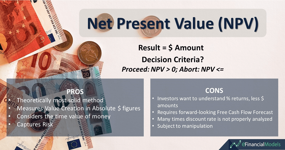
Net Present Value (NPV) is the difference between the cash inflows’ present value and outflows over a specified time. The specified time is usually the expected investment period. NPV analysis is one of the standard financial analysis methods to evaluate if a new investment project generates positive present value or not in $ amount. If the NPV is greater than zero or positive, the investment or project is highly likely to generate more cash inflows than outflows and is profitable. On the other hand, if the NPV is zero, below zero, or negative, the investment or project is expected to create fewer cash inflows than outflows and is, therefore, not profitable.
NPV is a widely used financial metric as it considers the time value of money and allows investors and businesses to make informed decisions about whether or not to invest in a project or opportunity. The NPV formula considers the time value of money, which states that money received today is worth more than money received in the future due to inflation and the opportunity cost of tying up capital.
How to Perform an NPV Analysis
NPV is calculated by discounting back cash inflows and outflows to their present value using a discount rate that reflects the time value of money. The formula to calculate the net present value is as follows:
NPV = [ Rt / (1+i)t ] – C
Where:
- Rt = net cash flow at time t
- i = discount rate
- t = time of the cash flow
- C = initial investment
NPV analysis requires a financial forecast of free cash flows typically over a minimum period of 5 years and including the terminal value at the end of the forecast period in year 5 (which captures the value from year six till eternity).
We will also need a discount rate that represents the opportunity cost of capital and is used to discount the forecasted annual cash flows to their present value as of today. Please refer to the article on how to calculate the WACC for estimating the discount rate. Alternatively, a discount rate calculator can help you discount the current value of future cash flows to the firm quickly and efficiently.
Below is a sample calculation using the NPV formula in Excel.
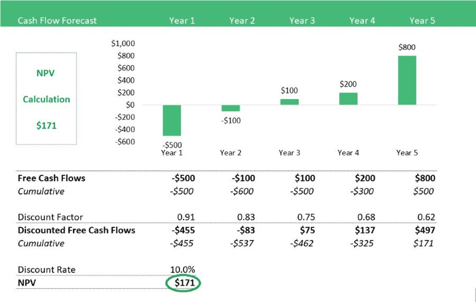
As you can see in the example above, if we would add up all the cash flows, we would obtain a value of $500. Because most of these cash flows ($800) occur in year 5, the discount effect is massive. Therefore, considering this all together, the NPV results in $171. When we examine the fundamental ideas of time and value, the point of the NPV analysis is that the further away a cash flow is in the future, the lower its value is today. It is because the time to carry uncertainty and risk will be longer for cash flows occurring in year five than in year one. This risk needs compensation in the form of a discount rate. The higher the discount rate, the higher the risk and the lower the cash flows in terms of their present value.
NPV is one of the most theoretically solid and forward-looking critical financial metrics. It measures value creation in absolute $ figures. The great thing about using it for financial decision-making is that it includes risk. Using NPV, new investment projects benefit if their risk is low but will be punished if an investor has to carry the risk for a long-time. It is one main advantage of using NPV for financial decision-making over alternative metrics such as payback period or return on investment calculations. The risk must be fully factored in, and an NPV analysis solves this.
Limitations arise if the quality of the financial forecast could be better or if the forecast reflects a subjective view of the future. Also, NPV results in a monetary amount but not a return metric, making it difficult to compare to other projects. Besides, investors typically want to understand % returns instead of $ amounts. As it requires a forward-looking free cash flow forecast, the discount rate may not be adequately analyzed or subject to manipulation.












































2) Internal Rate of Return
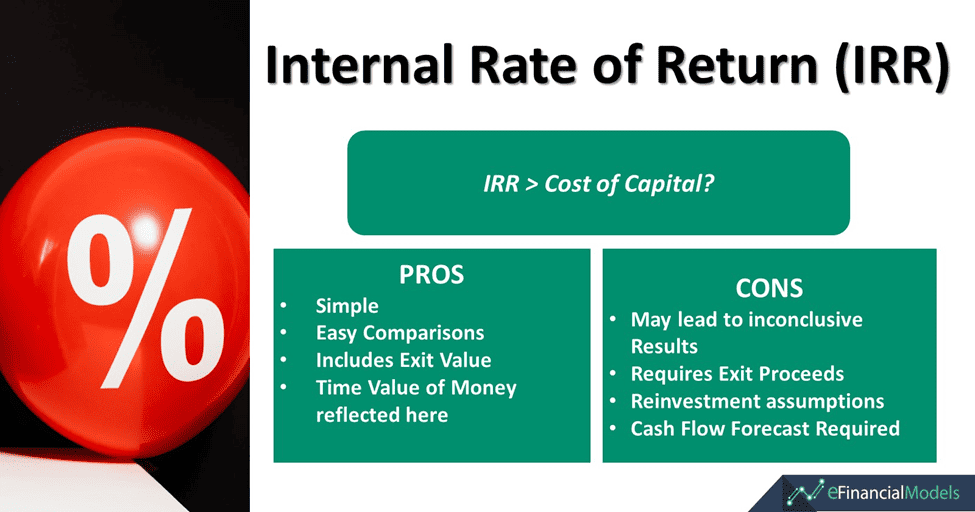
The Internal Rate of Return (IRR) tells you the expected annual return of a new investment project reflected in percentage. It may use the same financial forecast, such as NPV analysis but will result in a percentage return rather than monetary value. IRR is the discount rate that makes the net present value (NPV) of all cash flows from an investment equal to zero. If the IRR of a project is higher than the cost of capital, then the project is considered profitable.
IRR Variations
There are two variations of IRR – levered IRR and unlevered IRR.
- Levered IRR is the IRR of an investment when considering the impact of debt financing. In other words, it feels the effect of interest payments and the principal repayment on the investment’s cash flows.
- Unlevered IRR is the IRR of an investment without considering any financing, assuming all investments are made through equity. In other words, it only feels the cash flows generated by the underlying asset itself without factoring in any external financing.
The choice between levered IRR and unlevered IRR depends on the purpose of the analysis. If the investor is considering taking on debt to finance the investment, then the levered IRR may provide a more accurate picture of the potential profitability of the investment. However, if the investor is only interested in the underlying investment without any consideration for financing, then the unlevered IRR may be more appropriate.
How to Perform an IRR Analysis
The formula for IRR can be expressed as follows:
IRR = r (1 + NPV₁ / CF₁)^(t₁) = r (1 + NPV₂ / CF₂)^(t₂) = … = r (1 + NPVₙ / CFₙ)^(tₙ)
Where:
- r is the IRR (unknown and to be solved for)
- NPV₁, NPV₂, …, NPVₙ are the net present values of cash flows at different periods
- CF₁, CF₂, …, CFₙ are the cash flows at different periods
- t₁, t₂, …, tₙ are the time periods
The IRR is the rate that satisfies the equation above. This equation is solved using iterative methods like trial and error or numerical optimization algorithms. So, the best way to get an accurate IRR value is through an IRR calculation form in Excel. As IRR is the discount rate leading to a zero NPV, we can demonstrate this using the NPV example above.
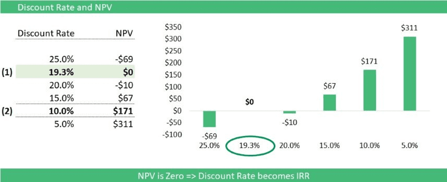
Instead of using a 10% discount rate, we increase the discount rate until we get to a discount rate that brings NPV to zero. As you can see in the chart above, this will happen when the discount rate is set at 19.3%; ergo, the IRR is 19.3%. So, what does this mean now? This project will generate a 19.3% annual return but also assumes that the cash flows received can be reinvested at the same rate.
IRR is a valuable tool for comparing different investment opportunities as it allows investors to determine which investment offers the highest possible rate of return. The advantage of IRR is that the analysis results in a return metric that can now be compared to the expected financial returns expected from alternative investment projects and also be compared to the required return in terms of the company’s cost of capital, estimated by the WACC. Investment projects competing for funding will often be compared and ranked by their IRR. (See example below)
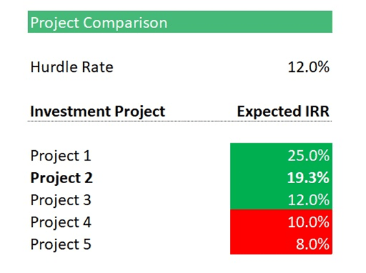
Commonly used in financial modeling to assess the viability of projects, it is compared to the cost of capital or hurdle rate of a project. As shown above, only 3 out of 5 projects are cutting off, producing a higher return than the company’s hurdle rate of 12%. Project 1 would even result in a higher IRR than Project 2, which now tells you to prioritize it. Therefore, IRR analysis becomes valuable when analyzing and comparing new investment projects.
In the context of exits, IRR is often used to evaluate the profitability of an investment in a private company, particularly when the investor is considering selling their shares. The IRR can provide insights into the potential return on investment, considering both the timing and size of the returns. All investments must be regarded as a whole, requiring extensive due diligence from all different angles. Investors use IRR because the metric is easy to calculate and understand.
It’s worth noting that while IRR is a helpful metric for evaluating investments, it does have limitations. IRR has some technical disadvantages, e.g., it only makes sense if it is possible to reinvest substantial cash flows at the same rate (reinvestment assumption) or if the cash flow pattern changes from positive to negative again, leading to an inconclusive calculation result. Cash Flows received earlier have a more significant impact on IRR than cash flows received later, which reflects the investor risk. Therefore, IRR is better suited to analyze buy and sell strategies rather than buy & hold, where substantial cash flows might only occur later. Similar to NPV analysis, IRR relies on the availability of a solid financial plan for at least five years into the future. It also requires a forward-looking free cash flow forecast that may be subjective.
Overall, the Internal Rate of Return is one of the key financial metrics used by professional investors, such as Private Equity Firms or Corporate Development departments, when preparing the basis for financial decisions.












3) Cash Yield
Another metric that investors may look at is the cash yield. It measures the annual return on an investment, expressed as a percentage of the initial investment. It considers the cash inflows and outflows associated with an investment, such as rent or dividend payments received, and deducts any related expenses or taxes. We can either look at the annual cash yield year by year, or we can compare the average cash yield over the expected lifetime of the planned investment. A cash yield should also aim to exceed a certain hurdle rate taking into account the nature and risk of the planned endeavor. Cash yield is mostly used by investors that are mostly interested in a buy-and-hold scenario and want to be assured that the returns are attractive so that the money is better kept here.
While both cash yield and IRR are measures of investment profitability, cash yield is focused on the annual return in form of free cash flows generated from an investment and might not include the exit value. When the cash flows are generated is less important as the annual cash yield makes no statement with respect to the time value of money. Cash yield is typically used for investments with stable cash flows, such as rental income or fixed-income bonds. Therefore, cash yield might not be suitable for certain industries which are subject to high risk and volatility.
In contrast, IRR considers the entire lifetime of the investment, takes into account the timing of the cash flows, and includes the exit value of an investment at the end. IRR considers the time value of money and can be used to compare investments with different cash flows over different periods.
How to Perform a Cash Yield Analysis
The formula to calculate cash yield is:
Cash Yield = Annual Net Cash Proceeds / Investment
Where:
- Annual Net Cash Proceeds: The net cash proceeds which can be created during one year. Net cash proceeds can refer to unlevered or levered cash flows depending on the definition used.
- Investment: The initial investment made. This either refers to the total investment or just the equity invested in a project.
We can demonstrate the calculation of the cash yield by using the example of the NPV calculation above. Only this time, we do not calculate NPV nor IRR, but we estimate the annual cash yield. (See example below)
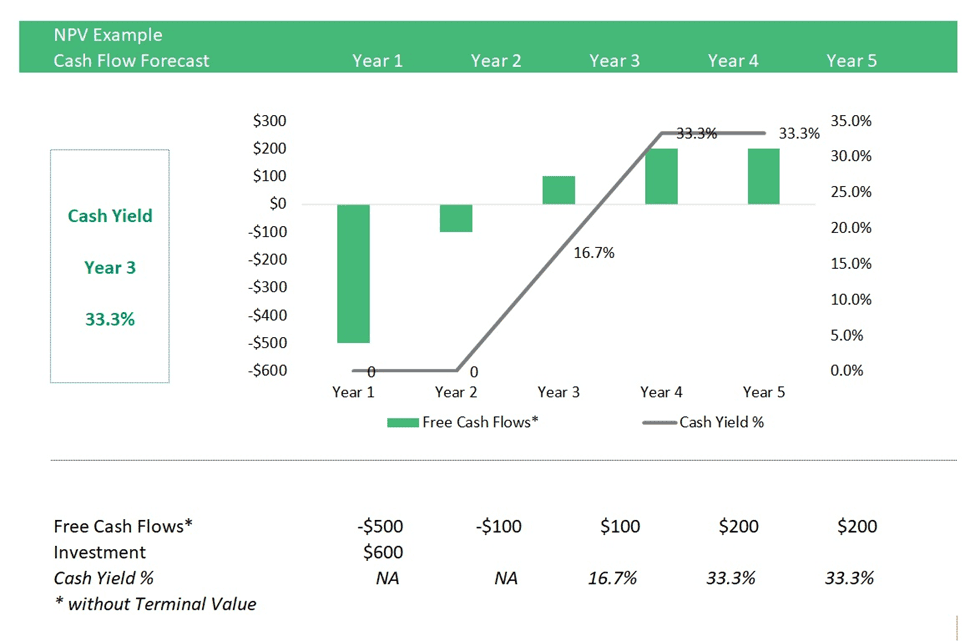
Initially, we invested $500 in year 0, but we also had to fund the operating loss in year 1. Therefore, the required investment is $600. The returns start to arrive as of the year, where we first expect to receive $100 and then $200 per year. Please note we are assuming a buy-and-hold scenario here. In the last year, we did not include the terminal value of $800 but an expected $200 annual cash flow (same as in year 4). As you can see below, the cash yield starts in year three at 16.7% and then rises to 33.3% annually.
The cash yield now tells us how much the return of an initial investment of $600 will be, assuming the asset will be held into the near future under a buy-and-hold scenario. Now we receive quite an interesting result since the IRR was “only” 19.3%. Still, when looking at the annual cash yield, which is higher at 33.3%, it would tell us that it would be a much better idea to keep holding this asset as it generates a higher yield than what we can get from a buy and exit scenario. Please note that no discounting is done in this case, and we look at real cash yields, which are still subject to risk. Furthermore, cash yield analysis only works for buy & hold scenarios. It measures what comes in in relation to what has been invested.
Cash yields can be calculated on an unlevered or levered basis per the investor’s preference. It is widely used in real estate investing, where you often have long buy-and-hold scenarios.

4) Payback Period
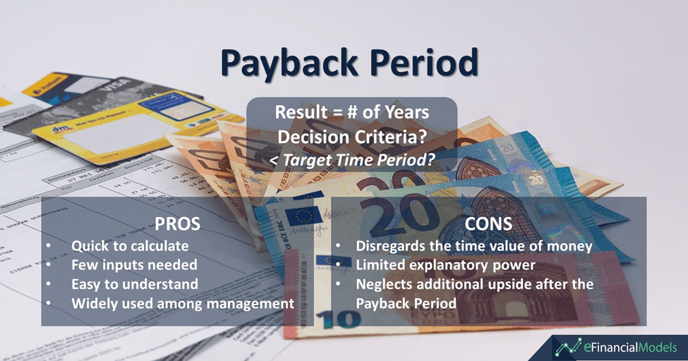
A financial metric called the payback period calculates how long a project will take to recoup its initial expenditure. It helps evaluate an investment’s risk, indicating how long it will take to become profitable. Payback analysis is a straightforward technique for assessing an investment project’s financial viability. It is a method commonly used by investors, financial professionals, and corporations to calculate investment returns. Typically, investors may have a target time period. A shorter payback period means a lower-risk investment, as the investor will recover their initial investment more quickly. You can use a payback period calculator to estimate the years to break even your investment quickly.
How to Perform a Simple Payback Analysis
The payback period is usually expressed in years, representing the time required to recover the initial investment. There are two formulas to calculate for the payback period.
If you are expecting even cash inflows for a project, the formula is:
Payback Period = Initial Investment / Expected Cash Inflow Per Period
For example, if your initial investment is $600 and you expect an annual cash flow of $300 every year:
Payback Period = $600/$300 = 2 years
For projects with uneven cash inflows, you must subtract the cumulative cash flows every year until they turn zero or positive. That means that the initial investment has already been covered. Let’s use the sample scenario in the cash yield calculation above. It shows that the project has an initial investment of $600 with the following anticipated annual cash flows:
Year 1 = ($500)
Year 2 = ($100)
Year 3 = $100
Year 4 = $200
Year 5 = $200
Let’s further assume the cash flow in Year 6 = $200.
To calculate the cumulative cash flow, we need to add the previous year’s free cash flow and the current year’s free cash flow. Please note that in Year 1, the initial investment will be our free cash flow for the preceding year. Here are the resulting figures.
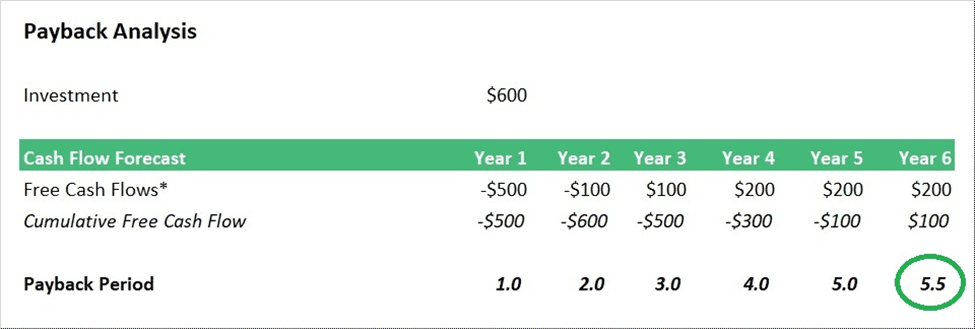
The table above shows that the payback period is 5 1/2 years. So, how do we arrive at the said figure? The formula we use is:
Payback Period = Previous Year that the Cumulative Free Cash Flow Turn Positive + (Cumulative Free Cash Flow of the Previous Year / 1st Positive Cumulative Free Cash Flow of the Previous Year)
In the example above:
Payback Period = 5 + (–$100/$200) = 5.5 years
It means that it would take five and a half years to recover the initial investment in the project.
The payback period is a simple method that does not require complex calculations or sophisticated financial models. The method needs few inputs and is relatively easier to calculate than other capital budgeting methods. It can be easily understood by non-financial stakeholders, making it a valuable tool for communicating financial information to a broader audience. If you want to quickly assesses a project’s financial viability, a payback analysis can be helpful in industries where time-to-market is critical.
But like any other method, the disadvantages of the payback period prevent managers from basing their decision solely on this method. One of its main drawbacks is that it needs to consider the time worth of money, a crucial business concept. According to the theory of the time value of money, money obtained sooner has a higher value than money received later due to the possibility of a higher return if reinvested. Such a technique needs to pay attention to this, which deviates from the actual value of the cash flows. Its focus is limited to the time required to recoup the initial investment and does not provide information about the project’s profitability or long-term viability. So, it neglects additional upside after the Payback Period. Furthermore, using the PBP technique, comparing and explaining projects across different organizations or industries may be limited.
Despite the disadvantages, the payback method is still used widely by businesses. The technique works well when evaluating small projects and projects that have reasonably consistent cash flows. Also, it is a go-to tool for small businesses, for which liquidity is more important than profitability.













5) Dynamic Payback Period
A more sophisticated and accurate method of evaluating the profitability of an investment is the dynamic payback period. The dynamic payback period considers the time value of money by discounting the expected cash flows back to their present value. The dynamic payback period calculates the time it takes for a project to generate enough discounted cash flows to recover the initial investment. As a result, the dynamic payback period provides a more accurate measure of the time it takes to recover an investment, as it considers the opportunity cost of investing in a project. However, it may require more complex calculations and assumptions about discount rates and cash flows, making it more challenging to apply in practice.
The dynamic payback period is generally longer than the payback period, as the dynamic payback period takes into account the time value of money, while the payback period does not. It means that the dynamic payback period provides a more accurate measure of the time it takes to recover the initial investment, as it considers the opportunity cost of investing in the project and the timing of the cash flows.
How to Perform a Dynamic Payback Analysis
The calculation for the dynamic payback period is the same as the formula for the payback period. The only difference is using the cumulative discounted free cash flow as the denominator instead of the cumulative free cash flow. To obtain the cumulative discounted free cash flow, you will need to multiply it with the discount factor for the said discount period.
Here’s an example:
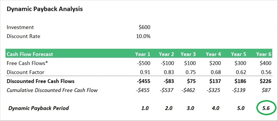
The figure above shows that the project had an initial investment of $600, with the following expected free cash flows:
Year 1 = ($500)
Year 2 = ($100)
Year 3 = $100
Year 4 = $200
Year 5 = $300
Year 6 = $400
Using the discount rate of 10%, we calculate the discount factor per year and multiply it by the free cash flow for the period. The cumulative discounted free cash flows are as follows:
Year 1 = ($455)
Year 2 = ($537)
Year 3 = ($462)
Year 4 = ($325)
Year 5 = ($139)
Year 6 = $87
The table above shows that the payback period is 5.6 years. So, how do we arrive at the said figure? The formula we use is:
Dynamic Payback Period = Previous Year that the Cumulative Discounted Free Cash Flow Turn Positive + (Cumulative Discounted Free Cash Flow of the Previous Year / 1st Positive Cumulative Discounted Free Cash Flow of the Previous Year)
In the example above:
Dynamic Payback Period = 5 + (87/$139) = 5.62 years
It would take around five years and seven months more to recover the initial investment in the project.
The dynamic payback period is simple to understand. It considers the time value of money by discounting the expected cash flows back to their present value. By discounting the expected cash flows, it considers the opportunity cost of investing in the project, providing a more accurate measure of the profitability of the investment. It can also help evaluate long-term projects with cash flows that occur further into the future.
Conversely, the dynamic payback period relies on accurate cash flow forecasts, which can be challenging to estimate, particularly for long-term projects. It also relies on a subjective discount rate, which can vary depending on the assumptions made by the evaluator. The dynamic payback period only considers cash flows until the initial investment is recovered, ignoring any cash flows beyond this point. As a result, it may provide a partial picture of the long-term profitability of the investment. Dynamic payback is more complex to estimate and explain than a simple payback calculation.
Overall, the dynamic payback period can be a valuable tool for evaluating the profitability of an investment, particularly for long-term projects. However, it is essential to carefully consider the assumptions made in the calculation, particularly when estimating cash flows and choosing a discount rate.
6) Cash on Cash (CoC) Multiple
Cash on Cash (CoC) Multiple is a financial metric used to evaluate the total return of an investment during its lifetime by using cash-in / cash-out consideration. This is mostly used in Private Equity or Real Estate Investment. A cash on cash multiple simply measures the total amount of cash received in comparison to the total investment made during the lifetime of a n investment project. The CoC multiple is calculated by dividing the total cash flow received from, e.g., a Property during a 5-year holding period by the total amount of cash invested in it. The resulting CoC multiple represents the amount of cash generated for each dollar invested in the property. It can be expressed as a multiple so that the CoC Multiple can be understood best.
How to Perform a Cash on Cash Multiple Analysis
The formula for Cash on Cash Multiple is:
CoC Multiple = Total Cash Flows/Initial Capital Invested during the Lifetime of an Investment Project
For example, suppose an investor made an initial investment of $600 in a venture and received a total of $1,800 in cash flows from that investment. The Cash on Cash Multiple would be calculated as follows:
CoC Multiple = $1,800 / $600
CoC Multiple = 3.0x
This means that the total cash flows received from the investment were three times the initial investment.
CoC is easy to calculate and understand. The metric focuses on the total cash flow generated by the investment property during the lifetime of an investment; ergo, it works better when a clear exit event is defined. The multiple offers a standardized way of comparing cash out versus cash in, making it easy to compare the potential returns of different investment properties.
One drawback of using the CoC multiple is that we need to know when the cash flows are coming in and capture the time value of money adequately. It is best used when comparing investments with similar cash flow patterns and holding periods, as it does not consider the timing of cash flows or the effects of compounding by itself.
Besides, it is overly simplistic. A Cash on Cash multiple of 3.0x could mean, [Example 1] we invest $100 today, and in 10 years, we get $300 back. We would also obtain the exact multiple if we invest [Example 2] $100 today and, for the next three years, receive $100 back each year (in total, $300). To know which example is more attractive to us, we would still need to use another metric such as IRR, which better reflects the time value of money.
Doing an IRR analysis would help us understand that the IRR of example 1 is better than the IRR of example 2 since the cash flows of Example 1 are received much earlier. One way to work around this is to consider the holding period an investment opportunity requires. It leads to a direct link between the Cash on Cash multiple and the IRR.
How is the Cash on Cash Multiple linked to the IRR?
As mentioned earlier, IRR analysis provides us with a solution to include the time value in a return percentage metric based on a forecasted stream of free cash flows.
What we can do now is to use the underlying cash in / cash outflows we were using to calculate the Cash on Cash multiple to simply also calculate the IRR. IRR assumes that cash returns can be reinvested at the same rate of return over time. This means when we know the target IRR, we will also know how much the cash multiple should be dependent on how long we are holding the investment until exit.
If you know the IRR and the number of years you will hold an investment, it is possible to compute the Cash on cash multiple of that investment by using the formula below:
Multiple =1*(1+IRR)^Years
Let us illustrate this with the following examples:
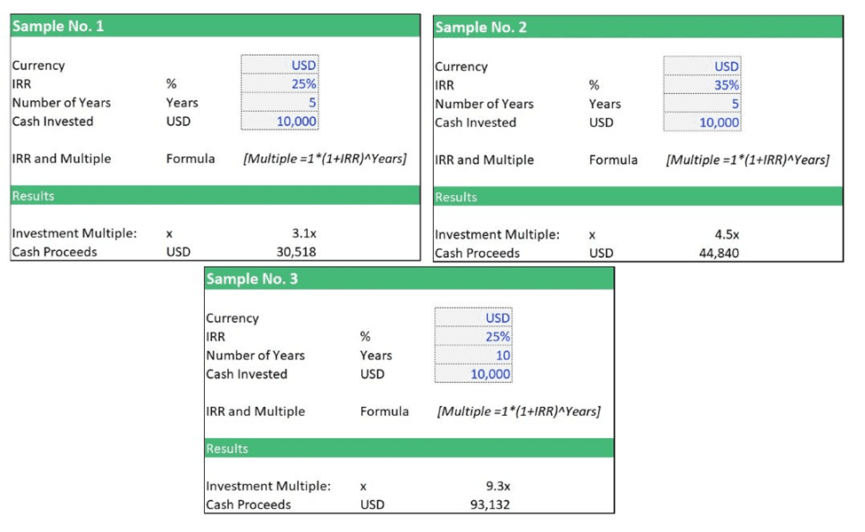
Under Sample No. 1, the IRR for five years will be 25%. The CoC Multiple will be 3.1x. In Sample No. 2, the IRR is assumed to be higher at 35%. If the return is higher, also the proceeds from reinvestment are higher, and that is why the CoC Multiple increases to 4.5x in Sample No. 2 (instead of 3.1x as per Sample No. 1). In Sample No. 3, the IRR remains at 25% (same as Example 1), but the investment period is extended to ten years. Now every year, the investment generates compounded 25% additional return. This leads to an increase of the CoC multiple to 9.3x.
To conclude, we can only understand the Cash on Cash multiple if we also understand the holding period. Larger holding periods have to result in larger cash on cash multiples. Otherwise, they would imply a lower IRR. CoC reacts when we increase the IRR and the planned investment horizon. The reason behind this is that the capital comes with the opportunity cost of capital, which require us to take into account the effects of compounding over time to ensure we are properly compensated for the risk.
A Cash on Cash multiple is quick to tell us how attractive an investment might be, but to understand the opportunity truly, we still need to understand the risk and the required investment horizon, and that is by doing an IRR analysis.

How to Know When to Use Which Key Financial Metric
As outlined above, each key financial metric comes with its pros and cons. Some are quick to calculate, while others are more difficult to calculate and require more parameters. Knowing which key financial metrics to use for your business case is essential to support sophisticated financial decision-making.
Financial analysis and planning require some understanding of these metrics to support your decision-making. Furthermore, it can also be a good idea to use more than one metric when running a financial analysis to avoid bias or overlook the potential limitations of each metric.
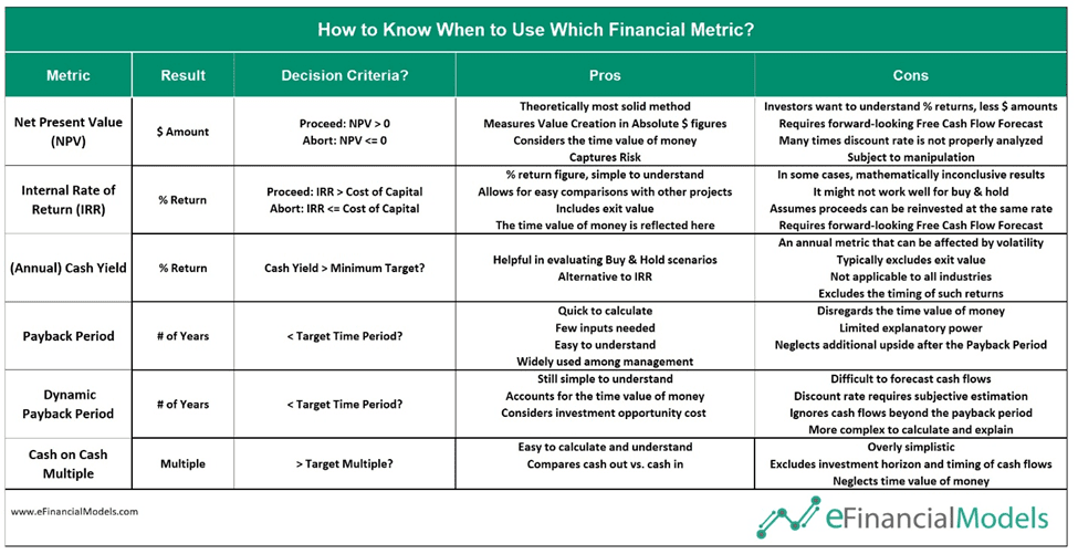
The following table compares the pros and cons of our suggested six key financial metrics:
Pro-Tips: Use one of our many financial model templates, which already include the calculation of one or multiple metrics above.
You might also like:
- 10 Ideas to Increase Average Revenue Per User
- Calculating Revenue Growth Rate: A Key Metric for Business Success
- What is Break-Even Analysis?
- 5 Smart Ways To Manage Personal Finances In A Pandemic
- 5 Tips to Develop a First Class Business Valuation Report
- Financial Ratios Analysis and Its Importance
- How to Build a Capitalization Table
- Understanding the Debt Service Coverage Ratio: An Essential Metric for Financial Analysis
- Strategic Insights to Secure Series B Financing
- 10-Step Financial Planning Checklist for Smart Executives
- Enhancing Financial Planning with Smart Metrics
- Financial Modeling for Startups and Small Businesses
- Personal Budgets
- Business Valuation
- Customer Acquisition Costs (CAC)
- Cash Flow Analysis
- Managing Days Receivable
- Market Metrics
- Traffic Count and Conversion Rate
- Investment