A ‘Rank’ represents a position in a hierarchy. Ranking is widely used- from politics to sports, from school grades to medical laboratories. The Rank Function In Excel displays a value’s respective rank compared to other values in a list. This is extremely helpful not only in evaluating data but also in summarizing key results.

Learning how to use RANK function in Excel is useful in sorting a business’s sales performance, expenses incurred per department, evaluating personnel performance, and assessing investments.

How Rank Function In Excel Works

The RANK function in Excel is a built-in function that determines the position (statistical rank) of a numerical value in a list of numerical values. It simply assigns a rank according to ascending (smallest to largest) or descending order (largest to smallest).

You use the RANK function in Excel when you want to know the ranking of a number in a list of numbers like the ranking for Sales for the Year, Expenses Incurred by Departments, Returns from Investments, etc.

RANK Function Syntax in Excel =RANK(number,ref,[order]

Where:

Number – The numerical value to rank.
Ref – Contains the numerical values to rank against Number. This can be a range of adjacent and non-adjacent cells.
Order – The [ ] brackets means this is an optional argument. This instructs Excel how to rank the list of numerical values in ascending or descending order. The RANK function in Excel has two ways of defining order, zero (0) and one (1).

• If you use zero (0) or if you leave this argument blank in the RANK formula in Excel, Ref follows a descending order. The largest numerical value in the list is ranked No.1
• If you use one (1) in the RANK formula in Excel, Ref follows an ascending order. The smallest numerical value in the list is ranked No.1.

Example of RANK formula in Excel
=RANK(F29,F$29:F$34,0)
=RANK(F29,F$29:F$34,1)

Example 1: How to use RANK function in Excel following a Descending Order.

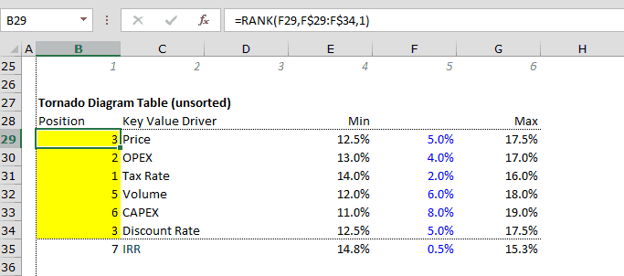
Assume below is your company’s key drivers, you can use RANK function in Excel to rank these from largest to smallest.

RANK formula in Excel =RANK(F29,F$29:F$34,0), Cell F29 represents the Number to rank, the cell range F$29:F$34 represents the Ref that contains the numerical values to rank against Number and 0 represents the Order of ranking.

Also, Cell F29 is relative (not locked and no $ sign) so the RANK formula in Excel adjusts to the cell position where the formula is copied and pasted. Whereas cell range F$29:F$34 is absolute, it will always refer back to these cell range regardless of cell position.

Example 2: How to use RANK function in Excel following an Ascending Order.

You can use RANK function in Excel to rank these key drivers starting from the smallest to largest.

Observe that RANK formula in Excel gives duplicate numbers the same ranking, notice that CAPEX and Price are both ranked No. 3 (essentially a tie). This affects the subsequent ranks, OPEX is ranked 5^th (instead of 4^th) and the Tax Rate is ranked 6^th (instead of 5^th). The rankings skipped the 4^th rank.

How To Use Rank Function In Excel For Unique Ranks (Break Ties)

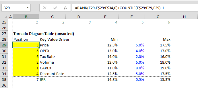
To rank a list and break any ties, we need to combine two functions- The RANK function in Excel is combined with COUNTIF function.

=RANK(F29,F$29:F$34,0)+COUNTIF(F$29:F29,F29)-1

The first part, the RANK formula in Excel, ranks the list as it normally does. So, it gives duplicate numbers the same rank.

The second part, COUNTIF function, breaks the tie in the rankings.

In the COUNTIF formula, the range is a single cell only (F$29:F29). The first reference cell is locked (F$29) and the second reference cell is relative (F29), meaning these changes based on the row where the formula is copied and pasted.

For as long as the numerical value appears only once, COUNTIF results in 1. The subtract 1 (- 1) at the end of the formula cancels itself out and restores the original rank.

But when duplicate numerical values appear, COUNTIF results in 2. The subtract 1 (- 1) at the end of the formula raises the rank by 1 only. This replaces the number’s rank that was skipped initially and so prevents duplicates to appear.

Crucial Tips On How To Use RANK Function In Excel

• When using the RANK function in Excel it is not necessary to sort the numbers on the list.
• RANK function in Excel only works with numerical values and does not recognize text.
• A RANKIF function in Excel does not exist to perform conditional rankings (greater than, less than, etc) similar to SUMIF and COUNTIF.
• #N/A! error happens when the numerical value to rank does not exist in the reference cells.
• In the latest versions (2010 and later) of Microsoft Excel, the RANK function has been replaced by RANK.EQ and RANK.AVG. The RANK function in Excel still works to enable backward compatibility, if you type the RANK formula in Excel it will display an exclamation point within the yellow triangle.

If you’re interested in how the RANK Function is used in a financial model, please feel free to download this Excel Template that utilizes the RANK Function in Excel.