Performing error checks in Excel financial models can be done in many ways. However, Excel also provides users with error handling functions. These functions catch, trap, and handle errors in Excel before these are displayed in your financial model.

One of these functions is the IFERROR function in Excel. If your formula in the financial model cannot locate the value it needs, wouldn’t it be better to display “Not found” versus #NA error? Or if a numerical input was mistakenly entered as text, wouldn’t it better to display it as a blank cell or a number zero versus #VALUE error?

In this article, we will answer the common questions about what IFERROR in Excel is, how to write the IFERROR formula, and when and how to use IFERROR in Excel.

What is the IFERROR in Excel?

The IFERROR function in Excel is part of the Logical functions and follows a TRUE/FALSE outcome. The IFERROR in Excel is designed to detect and isolate errors thus giving you the freedom how to best handle and troubleshoot errors.

To understand how to use IFERROR in Excel, it is best to briefly mention the IF function.

The IF function is a simple Logical function and works as follows:

1. Evaluates or tests data, formula, or expression based on given criteria
2. Depending on the outcome of the test,  it performs a specific course of action otherwise an alternative course of action

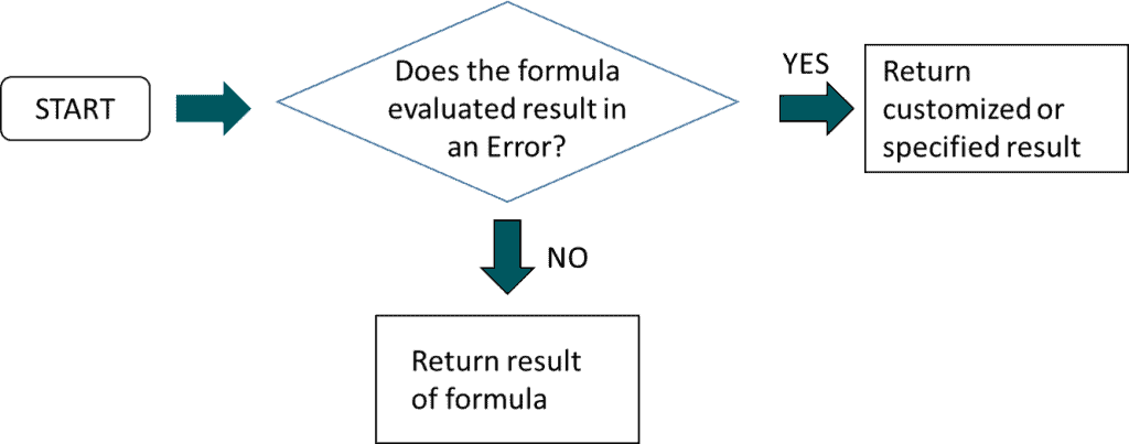
The IFERROR in Excel works in the same way. The IFERROR formula evaluates whether a formula’s calculation in Excel results in an error or not.

How Do You Write an IFERROR Formula?

The IFERROR formula is simple and straightforward, it is a good substitute to capture errors and manipulate the result without turning to complicated IF statements.

IFERROR formula in Excel:

Where:

Value
– The value that needs to be tested or checked for error (required argument). A reference cell or another formula is commonly used.
– If the Value argument is a reference cell and is not an error THEN this value is returned.
– If the Value argument is another formula and its calculation does not result in an error THEN its resulting value is returned.

Value_If_Error
– The value to return if an error is detected (required argument).
– The value to rerun can be expressed as a text string such as “Not Found”, “No data available” and can be a call to action like “Please input valid data”. It can be numerical such as the number zero (0) or simply a blank cell (“ ‘”). You can also instruct Excel to perform another calculation.

In simple terms, the IFERROR formula evaluates whether the Value argument results in an error. If it does then return the Value_If_Error argument otherwise return Value argument’s result.

When Do We Use IFERROR Formula in Excel?

When you want to test, eliminate, and replace errors in Excel financial models then IFERROR in Excel is the function to use.

When there are no errors, normally the formulas and functions in a financial model calculate and performs just as it should. But, when the results are errors the IFERROR function in Excel takes over and gives an alternative result.

When the following errors below occur, you can use the IFERROR formula to return an alternative result.

• #DIV/0!
• #NAME?
• #NA!
• #NUM!
• #NULL
• #REF!
• #VALUE!

How to Use IFERROR in Excel with Examples

Errors in Excel spreadsheets can be captured or handled using IFERROR function in Excel, these can be replaced by returning a blank cell, the number zero (0), or a customized message such as “Not Found”.

IFERROR in Excel Example 1 Return Blank

You can simply choose to leave a cell blank instead of displaying any error in Excel. Input the function name and an empty string represented by (“ “) as the Value_If_Error argument of the IFERROR formula to the original formula.

For example, to replace the #VALUE! Error in cell L5 the new formula with the IFERROR formula in Excel is:

=IFERROR($F5/$H5,” “)

The Value argument, ($F5/$H5), is the original formula. The IFERROR formula in Excel evaluates whether this returns an error or not. Since it returns an error, then the Value_If_Error argument represented by  (“ “) will display a blank cell.

Take note the IFERROR formula in Excel works with any error type in Excel. You can apply the IFERROR function in Excel to #NA and #DIV/0 errors.

IFERROR in Excel Example 2 Return Zero (0)

You can also use the IFERROR formula to replace errors with the number zero.

Using the same example, the new formula with the IFERROR formula in Excel is:

 =IFERROR($F5/$H5,0)

The IFERROR formula in Excel evaluates whether the Value argument ($F5/$H5) which is the original formula returns an error. Since it returns the #VALUE! Error, then the Value_If_Error argument represented by the number zero will display 0.

IFERROR in Excel Example 3 Return ‘Not Found’

Some errors may require a much more specific result other than zero or blank cells. For example, if your financial model looks up values from a reference sheet and cannot find the value then you can opt to display an alternative error message to #NA error.

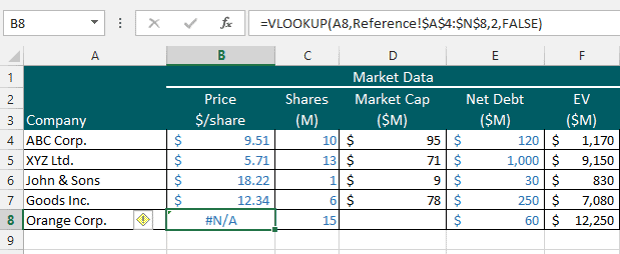
To illustrate, notice Price Column below uses the VLOOKUP function to look up the dollar share price value of a company from a separate sheet called Reference.  When the VLOOKUP function cannot find the price value for a company, it returns the #NA error.

An alternative or perhaps better error message would be to display the text “Not Found”.

The new formula with the IFERROR formula is =IFERROR(VLOOKUP(A8,Reference!$A$4:$N$8,2,FALSE),”Not Found”

The IFERROR formula in Excel evaluates whether the Value argument, the original formula VLOOKUP(A8,Reference!$A$4:$N$8,2,FALSE),  returns an error. Since it returns the #NA! error then the Value_If_Error argument represented by the text string “Not Found” will be displayed.

Proper Practices using IFERROR Function in Excel

• Hiding a true error in your financial model can lead to costly decisions so don’t catch or trap errors just because. Always use the Excel error check and create error checks specific to your financial model.
• To catch and handle specific errors with the respective course of action, use the following functions:
  • IFNA to catch #NA errors only and replace it
  • ISERR to catch all errors except #NA error but without replacing it
  • ISERROR to catch all errors but without replacing it