
0 ITEMS

Ten Ways to Estimate Terminal Value in DCF

Discounted Cash Flow (DCF) Valuation is the most used and theoretically sound valuation method for determining the expected value of a business based on its projected free cash flows. The DCF valuation method consists of two periods – the explicit forecasted period and the terminal period.
The explicit forecasted period consists of the free cash flows, projected long enough for a business to reach a steady state, typically five years. Exceeding the explicit forecasted period is the terminal period. The terminal period is based upon a financial principle – going concern, that companies have an unlimited lifetime.
- Accurate sales and expense estimates form the foundation of a reliable cash flow forecast.
- Regular updates reflecting actual performance help identify cash shortages early.
- Understanding seasonal fluctuations and business cycles improves forecast accuracy.
- Using digital tools like spreadsheets automates calculations and provides real-time insights.
- Conservative estimating and scenario planning build resilience against unexpected financial shifts.
Terminal Value represents the business’s estimated continuing enterprise value beyond the explicit forecast period. This article focuses on discussing the ten different ways to estimate Terminal Value and illustrating how to calculate the Terminal Value of a company.
In a standard Discounted Cash Flow (DCF) Valuation, Terminal Value generally contributes a significant portion to the Enterprise Value. In many cases, 60% – 70% of the Value is derived from the Terminal Value in a DCF Valuation model. Illustrated below is the most used and popular Terminal Value Method – the Gordon Growth Model, where its Terminal Value is 73.5% of the Enterprise Value.

Since Terminal Value significantly impacts the Enterprise Value, business valuation experts must analyze a company’s business case carefully when determining which Terminal Value formula to use. There are several other factors of importance aside from just the growth rate
Many times, only the Gordon Growth formulas come to mind when determining the Terminal Value. In this article, we would like to show that there are many more alternatives to consider than just using a standard Gordon Growth model for determining the Terminal Value in DCF.
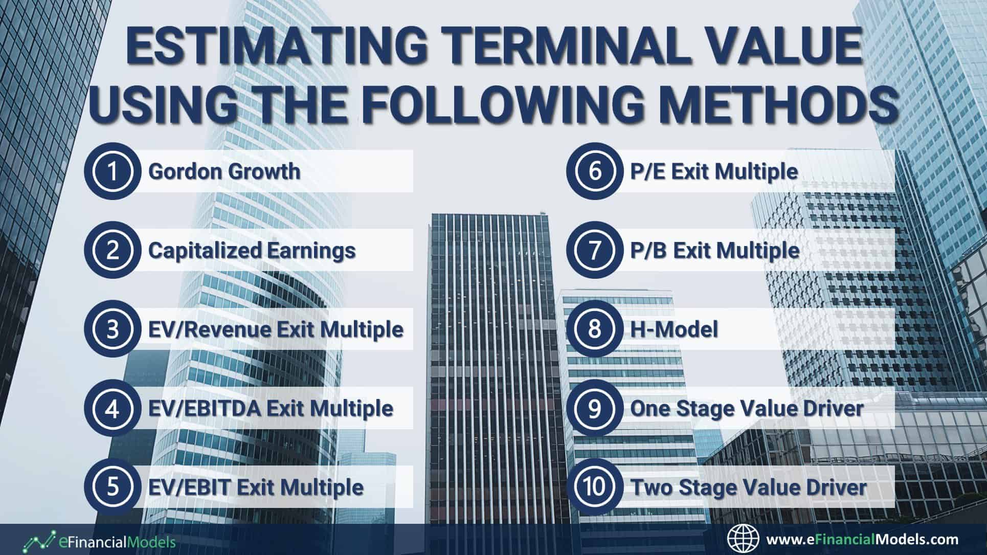
Ten different terminal value formulas and calculations are presented and explained hereunder to illustrate how each can be used and what difference they will make toward a DCF Valuation.
Follow the calculations outlined in this article by downloading the Advanced Version of the Discounted Free Cash Flow Valuation model (for FREE).
Different Methods for Calculating Terminal Value in DCF
Gordon Growth Formula
The Gordon Growth Model is one of the most widely used methods for calculating Terminal Value in DCF. It offers a quick and simple method to use, requiring only a few parameters for determining the terminal value:
- Normalized Free Cash Flows (at the end of the Forecast Period)
- Discount rate (WACC)
- Growth rate.
This terminal value method assumes that the normalized Free Cash Flows (FCF) of a mature, stable company will grow steadily at a long-term growth rate.
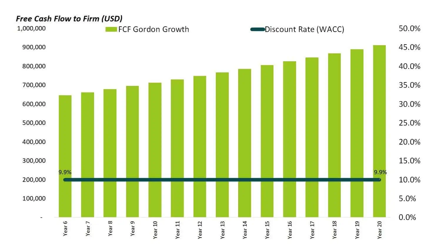
The growth rate is attached to the forecasted cash flows of a company after the explicit forecast period to determine how these cash flows are expected to grow in all future years. The long-term growth rate assumption generally is assumed to lie close to or slightly above the expected inflation rate.
Where:
FCFTV – Free Cash Flows at the end of the explicit forecast period of a five-year financial plan
WACC – Weighted Average Cost of Capital or the discount rate
g – Constant growth rate of FCF
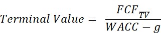
The Gordon Growth Terminal value formula is as follows:

Understand WACC further by visiting this link: Calculating the discount rate for Discounted Cash Flow Analysis.
Using the Free Discounted Free Cash Flow model template, the terminal value under Gordon Growth is calculated as follows.

The Gordon Growth Formula is one of the most widely used Terminal Value formulas and is also taught at the University Level. The formula is easy to use and only requires a few parameters to estimate Terminal Value. It is based on Free Cash Flows. In practice, however, the formula is overly simplistic, neglects, and includes unrealistic excess returns if ROIC is much higher than the WACC. Read more about the Gordon Growth formula to understand why it is the simplest yet restricted terminal value method.
Capitalized Earnings Method
Capitalized Earnings is also one of the simplest models for estimating the terminal value among the available valuation techniques. This method capitalized the Net Operating Profit Less Adjusted Taxes (NOPLAT) by the Weighted Average Cost of Capital (WACC) to arrive at the Terminal Value (TV).

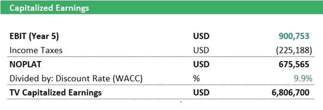
Please note that here we are capitalizing NOPLAT and not Free Cash Flows. Same as the Gordon Growth Formula, the formula is simple to use but lacks analysis and explanatory power.
Calculate the Terminal Value under the Capitalized Earnings model using the Free Discounted Free Cash Flow Model Template.
EV/Revenue Exit Multiple
An Exit Multiple Approach, in general, may be used as a valuation metric to quickly calculate the value of a business relative to a financial reference metric. This approach is quite simple and straightforward to apply.
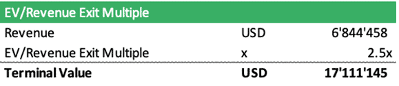
One common Exit Multiple is the EV/Revenue Multiple. EV Stands for Enterprise Value, while revenue reflects the company’s annual net revenue of the last explicit forecast year 5. The multiple can also be observed on the stock market by calculating the implied relationship between a company’s revenues and its Enterprise Value (Market Capitalization + Net Debt).
Terminal Value = Revenue * EV/Revenue Multiple
Please note that in this case, the calculated Terminal Value corresponds to the Enterprise Value in Year 5. The chart shows how Terminal Value can be calculated using this method:
There are several advantages of using an EV/Revenue multiple to calculate Terminal Value. The multiple is quick to calculate and can be compared to the implied valuation of publicly quoted companies. Revenue as a top-line figure is least subject to distortion or manipulation by accounting gimmicks. In cases where a company still will be running a loss instead of being profitable at the end of the forecast period, other multiples might not work. Still, an EV/Revenue multiple can offer a solution to estimate Terminal Value in such cases.
The main disadvantage of using an EV/Revenue multiple, in this case, is that it completely disregards a company’s cost structure and profitability situation. This opens room for critique and will lead to a more significant degree of inaccuracies than e.g., using an EV/EBITDA multiple for calculating Terminal Value.
EV/EBITDA Exit Multiple
EBITDA stands for Earnings before interest, taxes, depreciation, and amortization. Using an EV/EBITDA multiple to calculate Terminal Value is very similar to using an EV/Revenue Multiple.
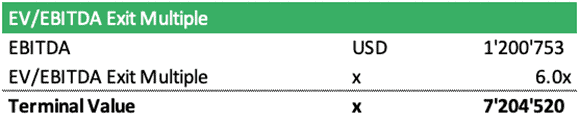
Terminal Value = EBITDA * EV/EBITDA Multiple
We calculate the Terminal Value (corresponding to the Enterprise Value at the end of the Forecast Period) by multiplying the EBITDA in the last forecast year with a selected multiple. The following illustration explains the calculation of Terminal Value:
The selected multiple should be researched based on publicly quoted companies’ implied valuations or observed multiples from recent transactions in the same industry.
The advantages of using an EV/EBITDA multiple in this situation are the following:
- Calculating Terminal Value based on an EV/EBITDA multiple offers a simple and easy-to-understand solution. Instead of having to explain and defend a complicated formula, EV/EBITDA multiples can be observed on the market. Therefore, it is easier to communicate its use to bankers, investors, or other stakeholders.
- Unlike Revenues, EBITDA is a profit figure; therefore, the company’s cost structure matters.
- EBITDA is calculated before considering depreciation and amortization, which sometimes are manipulated by the management to look good (window dressing). EBITDA is the closest cash profit figure you usually can get.
- EBITDA is also the preferred valuation multiple to value private company transactions by Private Equity firms. Highly accepted by investors and other stakeholders, buyers indeed would value the company in five years based on an EV/EBITDA multiple.
Of course, there are also some disadvantages of using an EV/EBITDA multiple to calculate Terminal Value:
- We can only apply an EV/EBITDA multiple if there is a profit. This raises the question of how much a company is worth if the company, by year 5, would still not profitable. Using an EV/EBITDA multiple either leads to an Enterprise Value of zero or even negative. However, if a company possesses valuable assets, then a buyer most likely would still be willing to pay something to acquire the company.
- EBITDA is unsustainable. A financial forecast could show a hockey stick business plan leading many times leading to a pro-forma EBITDA which reflects unusually high EBITDA margins or an unusually high Return on Invested Capital (ROIC). Based on experience, such high margins are not sustainable, and potential buyers, for that reason, might not be willing to pay a market multiple.
- The value of tax optimization achieved does not matter. This contrasts with a Free Cash Flow based Terminal Value valuation method where Free Cash Flows benefit from a low tax rate.
Overall, using an EV/EBITDA multiple offers a simple and straightforward solution to calculate Terminal Value in most cases.
EV/EBIT Exit Multiple
EBIT stands for measuring profits before interest and tax expenses (Earnings before Interest and Taxes). If, for some reason, EBIT is viewed as a better profit measure than EBITDA, using an EV/EBIT multiple can offer another alternative to calculate Terminal Value. Same as EV/Revenue and EV/EBITDA multiples, the EV/EBIT multiple calculates Enterprise Value.
Terminal Value = EBIT * EV/EBIT Multiple
The calculation is very similar to using an EV/EBITDA multiple, only that normally, EV/EBIT multiples are higher than EV/EBITDA multiples when valuing the same company (since EBIT is after depreciation and amortization).
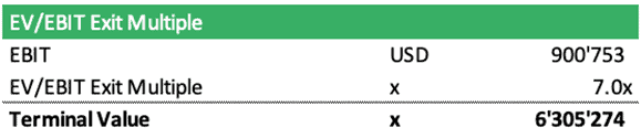
Identical to the EV/EBITDA multiple, using an EV/EBIT multiple is easy to explain, and the EV/EBIT multiple approach only works if the company is profitable. Then the main problem here is that the multiple very often is subject to manipulation as depreciation and amortization expenses are deducted. Depreciation and amortization expenses are non-cash costs that must be estimated based on an asset’s useful life (number of years). Furthermore, many times the management team can also choose whether to depreciate faster in the early years than in later years or vice versa. All these choices offer much room for management to manipulate these non-cash expenses; therefore, EBIT becomes distorted.
P/E Exit Multiple
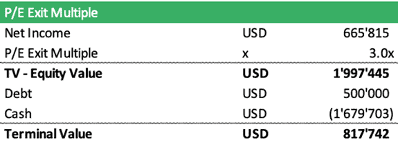
Another alternative to calculating Terminal Value is using a Price to Earnings (P/E) multiple. Typically, the P/E multiple is calculated on a per-share basis. The formula can be modified to calculate a target Market Capitalization by multiplying Net Income with a P/E Multiple. The Target Market Capitalization corresponds to the market value of the Equity. Therefore, the following formulas apply:
Value per Share = Earnings per Share x P/E Multiple
Equity Value = Earnings per Share * Number of Shares Outstanding x P/E Multiple
Equity Value = Net Income x P/E Multiple
However, Terminal Value needs a figure corresponding to the Enterprise Value. Thus, Net Debt is added to the Equity Value to calculate the Enterprise / Terminal Value. Net Debt is calculated as Financial Debt – Cash and equivalents.
Enterprise Value = Equity Value + Financial Debt – Cash
Terminal Value = Enterprise Value
The following example illustrates the calculation of Terminal Value using a P/E multiple:
Using a P/E ratio comes with its pros and cons:
Pros:
- Net Income reflects the bottom-line profits and includes all and every cost.
- P/E ratios typically are observed in the stock market, and many financial data pages provide this ratio readily calculated.
- P/E Multiple is often used as a quick way to value stocks; therefore, many investors are already familiar with it, and it should be pretty simple to explain its use. Many investors also remember a rule of thumb that in the long-term, a P/E multiple normally balances towards 15.0x at the stock market.
- The multiple only works for valuing profitable companies since a Negative Net Income by year 5 leads to a negative or close to zero Equity Value.
Cons:
- Net Income is a pure accounting figure and even more distorted than EBIT. It is nowhere near a cash-like profit figure and, therefore, often subject to manipulation and accounting rules.
- Using a P/E Multiple calculates Equity Value and not the Enterprise Value, which is needed for Terminal Value. Problems arise if a company has excess cash on its balance sheet by year 5, which can severely impact the valuation.
- When using DCF as a means to conduct fundamental analysis, the analysis should prefer the use of Free Cash Flows. Using a P/E multiple is pretty much the opposite. Therefore, it can reduce the explanatory power of the DCF analysis and open room for critique.
In general, P/E ratios are rarely used for calculating Terminal Value in a DCF valuation analysis for the reasons mentioned in the Cons. However, in an exceptional case, using a P/E ratio could still offer an alternative way of calculating Terminal Value if needed.
P/B Exit Multiple
As mentioned above, many profit-related multiples, such as EV/EBITDA, EV/EBIT, and the P/E ratio, only work if the company is profitable. For asset-intensive companies with low profitability, another way will be needed to estimate the Terminal Value.
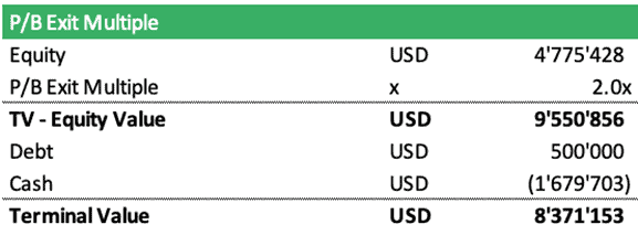
Here is where the Price to Book (P/B) ratio comes in. It estimates the value of a business based on the relationship between the Market Value of Equity and its Book Value which translates into the P/B ratio. Same as the other multiples, the P/B ratio can also be observed on the stock market when analyzing the implied valuations of publicly quoted companies. Here is how the P/B formula is applied when calculating Terminal Value:
Equity Value = Equity Book Value * P/B Ratio
Enterprise Value = Equity Value + Financial Debt – Cash
Terminal Value = Enterprise Value
The example below illustrates how Terminal Value can be calculated based on a target P/B ratio:
The main advantage of using a P/B ratio to calculate Terminal Value is that it allows for valuing of capital-intensive businesses which do not show many profits. However, this lack of considering the profit aspect in the valuation is also one of this technique’s main weaknesses, which opens room for critique. Another weak point is that the ratio uses Equity Book Value, whose calculation depends on accounting standards, making it nearly impossible to compare apples with apples when using P/B ratios from similar companies in other geographies.
H-Model
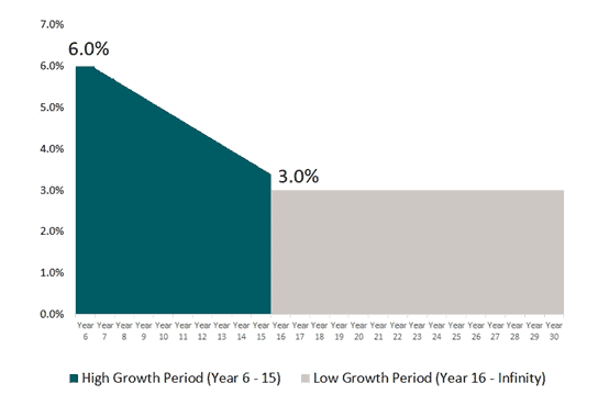
The H-Model can be viewed as an upgraded version of the Gordon Growth Model. The main problem with the Gordon growth model is that it is very simplistic. If a company shows periods of strong growth, a more fine-tuned formula is needed to capture periods of high growth and the period of long-term growth. The H-Model depicts growth in two phases starting as of year 6 (first Terminal Value year in a DCF Valuation analysis) with a high growth rate:
- A period that starts with a High-Growth rate that declines to a long-term growth rate
- Period of long-term growth
The H-Model splits the Terminal Value years into two phases where cash flows grow at different growth rates. The chart below shows an example. Growth is expected to start at 6.0% in the first period and then decline to the growth rate of the second period, which reflects a long-term growth rate.
Below are the assumptions needed to estimate Terminal Value by using the H-Formula:

FCFTV – Free Cash Flows at year-end of the forecast period (Year 5)
WACC – Weighted Average Cost of Capital or the discount rate
gL – Low growth rate of FCF
gH – High growth rate of FCF
H – Number of Years of High Growth divided by half
Terminal Value using the H-Formula is calculated as follows:
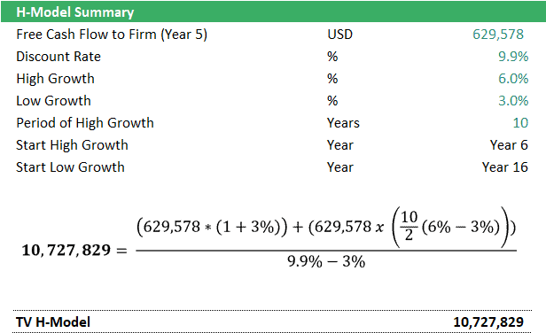
Compared to the Gordon Growth Model, the H-Model allows for fine-tuning the phases of high-growth and low-growth better. That being said, there are a bit more parameters needed for the H-Formula. One weakness of the H-Formula is that the focus is on growth as the primary value driver. The business’s future profitability and how much capital is required are also neglected. Therefore, the formula is simplistic and not used often for calculating Terminal Value.
Learn more about why the H-Model considers different growth periods for calculating Terminal Value.
One Stage Value Driver Formula
As explained above, the other Terminal Value formulas try to simplify reality by primarily putting one aspect in the center when calculating Terminal Value, which is typically the growth rate.
A One Stage Value Driver Model now introduces a second key value driver, which is the: Return on Invested Capital (ROIC). The ROIC measures the profitability from every dollar invested into a business. The higher the ROIC, the more valuable an investment becomes. The lower the ROIC, the more capital needs to be invested for a given amount of return. Value Driver models now allow the definition of a target ROIC that a business should achieve over time.
A One-Stage Value Driver Model focuses on modeling terminal value based on the target profitability this business should generate in the long term, and the ROIC reflects that target profitability. Terminal Value is now calculated based on the relationship between the discount rate, the terminal growth rate, and the investment needed to reach that growth.
The following Terminal Value formula applies:

FCFTV – Free Cash Flows at year-end of the forecast period (Year 5)
WACC – Weighted Average Cost of Capital or the discount rate
g – Growth rate
NOPLAT – Net Operating Profit less Adjusted Taxes
ROIC – Return on Invested Capital
Let us look at how this formula is applied in the example computation below:
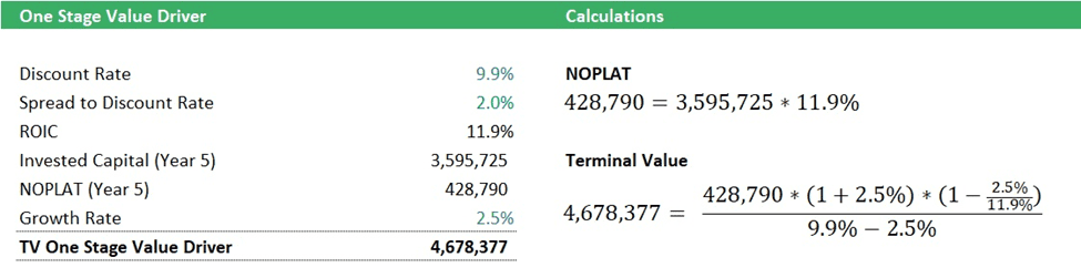
In the above example, ROIC is defined through a spread to the Discount Rate (WACC). A spread of 2.0% means the company is expected to generate an annual profit of 11.9% of every dollar invested into the business. In comparison, the required returns of companies with similar risks lie at 9.9%. This business is expected to benefit forever from a slight competitive advantage, resulting in an excess return of 2.0%. The growth rate g still plays a role, but growth is not solely the determinant of the resulting value in the Terminal Value model anymore.
The advantage of using a value driver model is that it is more realistic to define the long-term expected ROIC of a business than only the growth rate. This formula also addresses the main drawback of the Gordon Growth model, which is that Free Cash Flows with abnormally high ROICs are included forever in the Terminal Value.
The weakness of using a One-Stage Value Driver Model is that another parameter is required: the ROIC. This terminal value model also tries to simplify reality by assuming a normalized pattern of Free Cash Flow Generation.
Read more about the One Stage Value Driver Model and how to use the formula to calculate the terminal value for a DCF Valuation.
Two Stage Value Driver Model
Finally, one of the most sophisticated approaches to model Terminal Value is the Two-Stage Value Driver Model. In contrast to the One Stage Model, the Two-Stage Model splits the Terminal Value period into two stages:
Stage 1: Period which generates excess returns as the company enjoys a competitive advantage
Stage 2: Period where the competitive advantage is gone, and the company will just generate market returns
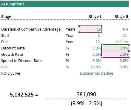
Instead of using a Terminal Value formula, an annual forecast is modeled for all the terminal value years year using the following assumptions:

As seen above, different ROICs and Growth rates can be assumed per Stage.
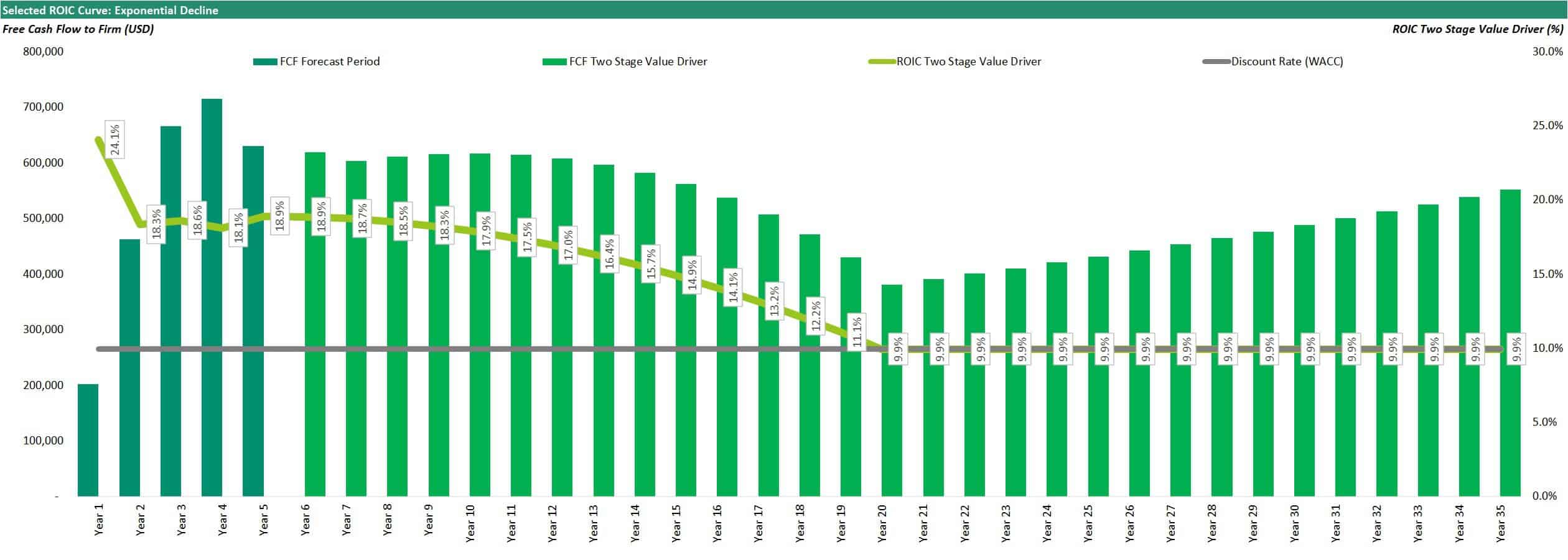
Stage 1 – Revenues are forecasted to grow at the envisaged growth rate as of stage 1 from year 6 to year 20 while modeling the ROIC to decrease from the target to the long-term ROIC in Stage 2. The forecast built is quite comprehensive so that users can understand the implied profitability, the invested capital, and the annual investments required.
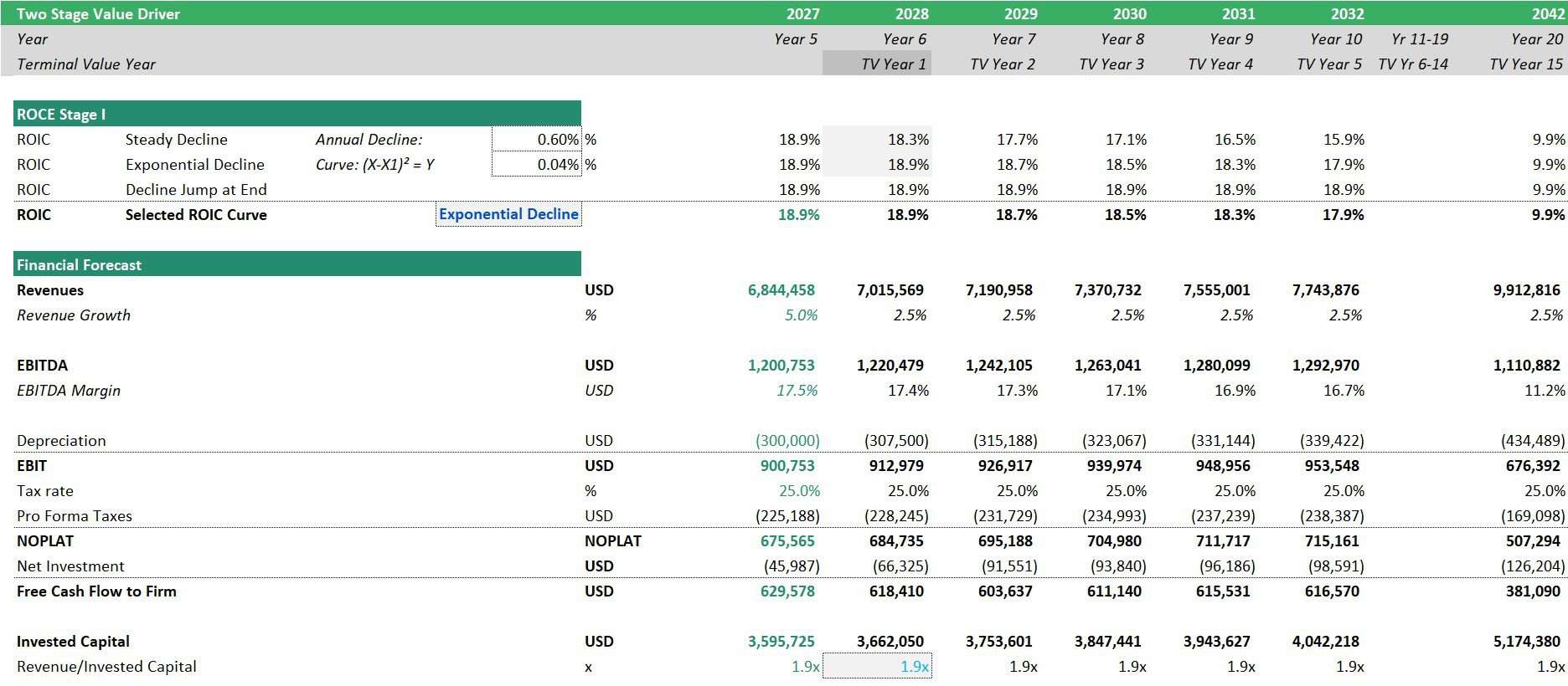
Free cash flows for the Stage 1 period are discounted.

Stage 2 – Once the competitive advantage period ends, from Stage 1, ROIC will decline to WACC (9.9%) or a target ROIC at the beginning of Stage 2 period.
Terminal Value at the end of the competitive advantage period is calculated using a Gordon Growth model – but this time, the cash flows correspond to a target ROIC – where:
FCFTV – Free Cash Flows at the end of the Competitive Advantage period
WACC – Weighted Average Cost of Capital or the discount rate
g – Growth rate

The chart below illustrates how the Two Stage Value Driver model drives ROIC down and the impact on Free Cash Flows. Free Cash Flows will grow on a lower level once ROIC returns the market return (same as the WACC).
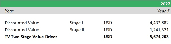
Modeling terminal value this way allows us better to capture the key value drivers of the business and come up with a more sophisticated argumentation of which cash flows the terminal value contains and how they have arrived. The terminal value under the Two Stage Value Driver Model is calculated by summating the discounted cash flows of the two stages.
This terminal value approach is unique, allowing users to view the length of the competitive advantage period – where the business can produce superior returns (ROIC>WACC) and focus attention on which ROIC and growth rate to include for both stages. From a fundamental point of argumentation, this approach is considered a more sophisticated method for determining the composition of the terminal value. Also, Free Cash Flows are not hidden in some hard-to-understand formulas but are explicitly stated in this model.
On the contrary, this approach requires more assumptions than, e.g., a Gordon Growth Terminal Value approach, which can produce new complications. Also, it is more challenging to model than a Gordon Growth formula
Understand further in the detail the phases in a Two Stage Value Driver Model by reading through the step-by-step process of estimating terminal value.
Comparing Terminal Value Formulas
The results of the ten different terminal value models are summarized in the illustration below. The dark green represents the Terminal Value as per the end of Year 5, while the data in light green shows the present value of the Terminal Value as per year 0.
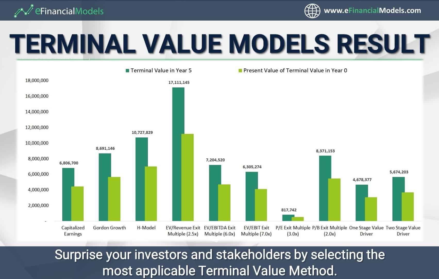
As demonstrated above, the resulting Terminal Value strongly depends on which formula and assumptions are used, which could open doors for manipulations of DCF valuations. The best protection to deal with that is to know the strengths and weaknesses of each Terminal Value formula.
Depending on which Terminal Value Formula is used, the impact of Terminal Value on the overall standard Discounted Cash Flow (DCF) Valuation result (Enterprise Value) significantly varies between 20% – 80% of the Enterprise Value.
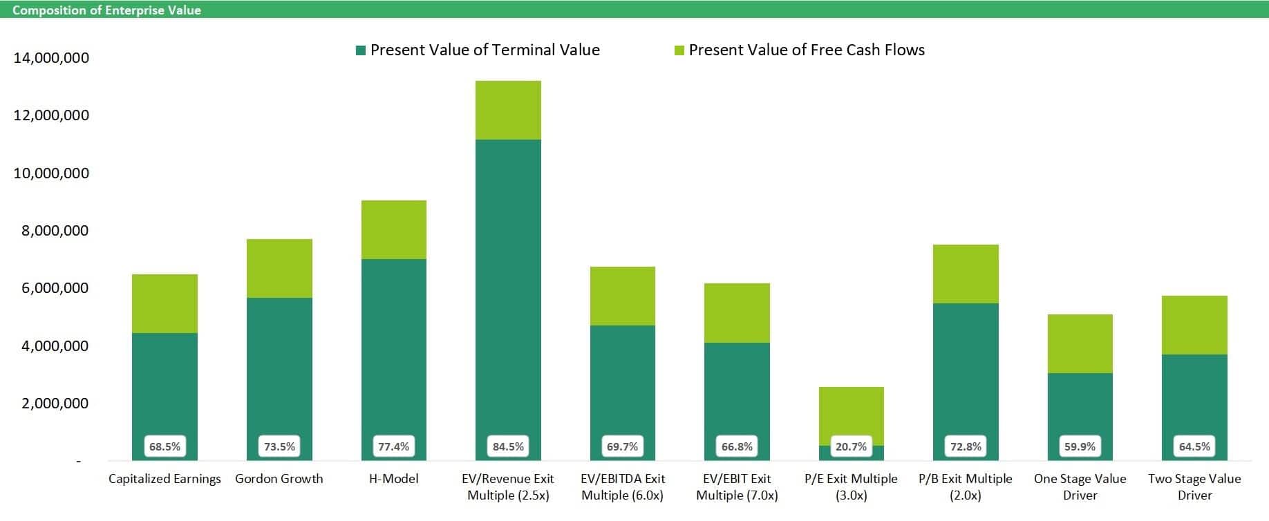
The result of each Terminal Value Model depends on assumed fundamental parameters in the formulas. Hence, the Terminal Value result highly varies depending on which method is selected. Based on the illustrations above, the EV/Revenue method led to the highest value, while the P/E multiple showed the lowest terminal value.
To conclude, it does matter which Terminal Value method and assumptions are used for business valuations.
Selecting the Terminal Value Method Matters
As discussed in this article, there is more than just one method to calculate Terminal Value. Business valuators can at least choose between ten different valuation methods, some simple, some more complex, to determine Terminal Value in a Discounted Cash Flow Valuation.
Each terminal value method focuses on selected aspects that drive value at the end of the forecast period. Not every method is suitable for all situations. A terminal value model should always be selected considering a company’s specific circumstances. The table summarizes the main pros and cons of each Terminal Value method.
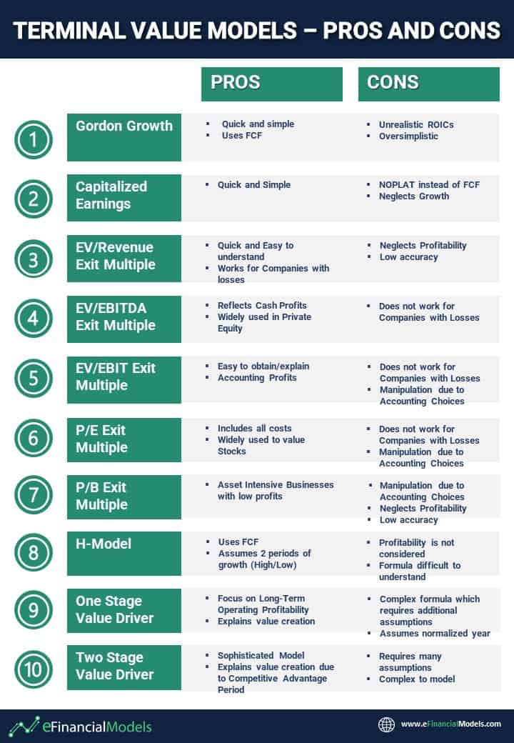
It is best to select those techniques that are the most relevant and reliable, depending on company circumstances and the readily available data.
Surprise your investors and stakeholders using one or more of the advanced Terminal Value methods presented in eFinancialModels’ Advanced Version of the Discounted Free Cash Flow Valuation model (for FREE).
In many cases, the opinion of a professional appraiser might be needed. Do not hesitate to contact our team if you need any assistance.
If you’re looking for financial model templates that include a DCF Valuation, please feel free to check out our full list of DCF Model templates here:























































- Value Your Business With the EV/Revenue Multiple
- 10 Steps to Create a Drop Down List Using Data Validation in Excel
- A Step-By-Step Guide to Economic Profit Calculation
- How to Calculate Net Present Value (NPV)?
- How to Calculate the Compound Annual Growth Rate (CAGR)
- Financial Analysis
- Financial Statements – Definition, Uses, Contents and Templates
- Accounting
- Unlocking The Full Potential of Meal Prep Business Plan PDF
- How to Make Smart Decisions with 6 Key Financial Metrics?
- Financial Project Management
- Financial Modeling for Startups and Small Businesses
- Real Estate
- 10 Tips to Develop a First Class Business Valuation Report
- 10 Awesome Excel Formulas To Use For Your Next Financial Model In Excel
- Financial Modeling Best Practices
- Why Do You Need a Financial Model?
- 5 Ways COVID-19 Impacts Financial Plans For Retirement & What To Do About It
- Understanding the Levelized Cost of Energy Formula
