
0 ITEMS

Bankable Macro Enabled Financial Model for Utility-Scale Solar PV Projects
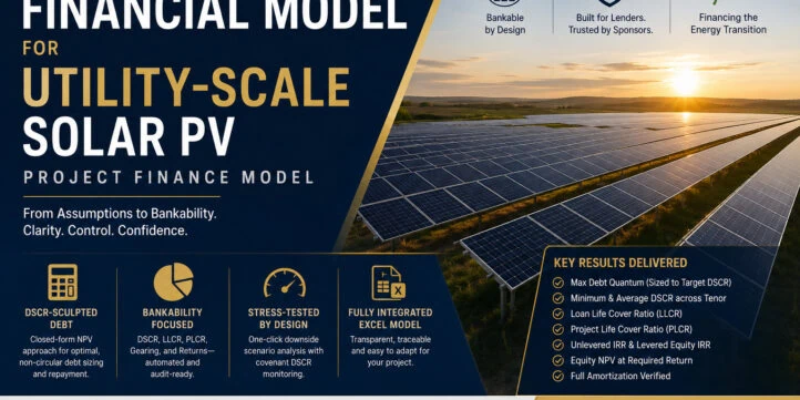
Bankable Financial Model for Utility-Scale Solar PV Project Finance This Excel-based financial model is a lender-grade project finance tool designed for utility-scale solar PV projects. It supports project developers, lenders, investors, financial advisors, and infrastructure sponsors in evaluating project feasibility, debt capacity, and equity returns using industry-standard project finance methodologies. The model follows a transparent, fully integrated workflow from engineering and commercial assumptions through to debt sizing, financial statements, and investment metrics. At its core is a DSCR-sculpted debt repayment methodology that sizes debt according to projected cash flows rather than using conventional fixed amortization schedules. This reflects best practice in project finance by aligning debt service with the project’s cash generation profile. The workbook comprises nine logically linked worksheets covering assumptions, energy production, revenue, operating costs, CFADS (Cash Flow Available for Debt Service), debt sculpting, equity returns, summary outputs, and stress testing. All user inputs are centralized, colour-coded, and easily traceable, allowing assumptions to be modified without altering model formulas. A key feature is the non-circular debt sculpting engine, which applies a closed-form Net Present Value (NPV) approach to calculate debt capacity while avoiding Excel circular references. This improves model stability, transparency, auditability, and lender confidence. The model automatically calculates annual debt service, principal repayment, interest, loan balances, gearing, and key credit metrics including DSCR, LLCR, PLCR, Project IRR, Equity IRR, and Equity NPV. An integrated Stress Test module enables rapid downside scenario analysis, including P90 production cases and covenant testing against a minimum DSCR threshold. A documented VBA macro allows users to re-sculpt debt under stressed cash flows without affecting the base-case model. The model is built around internationally recognised project finance principles and is intended as a robust, extensible template suitable for adapting to project-specific assumptions, jurisdictions, tax regimes, financing structures, and offtake arrangements. While the default assumptions are illustrative, the framework can be readily customised for real-world transactions, making it an excellent foundation for feasibility studies, lender due diligence, investment analysis, and bankable financial modelling.
A Bankable Financial Model for Utility-Scale Solar PV Project Finance
Overview
This workbook is a full-stack project finance model for a utility-scale solar photovoltaic (PV) generation asset, built to the standard expected by lenders, their technical and financial advisors, and equity sponsors evaluating a greenfield or acquisition opportunity. It takes a project from a single set of engineering and market assumptions through to the two numbers everyone in the room actually cares about: how much debt the project can support, and what return equity holders can expect to earn for taking the risk that sits behind that debt.
The model is deliberately built around one central design choice: debt is sculpted, not amortized on a flat schedule. Rather than assuming a level annuity repayment (as a mortgage would), the model sizes principal repayments year by year so that the project’s debt service coverage ratio (DSCR) sits at a lender-specified target in every period the constraint binds. This is standard practice in project finance because project cash flows are rarely flat — solar output degrades gradually every year, operating costs escalate with inflation, and revenue profiles can shift under time-of-day or seasonal pricing. A sculpted structure lets the debt quantum flex to match the shape of the cash flow, rather than forcing the project to hold a large cushion in early years and a thin one in later years, or vice versa.
Structure of the Model
The workbook is organized as a logical chain of nine sheets, each doing one job, so that a reviewer can trace any number in the summary output back to its underlying assumption without switching between disconnected files or hunting through a single monolithic sheet.
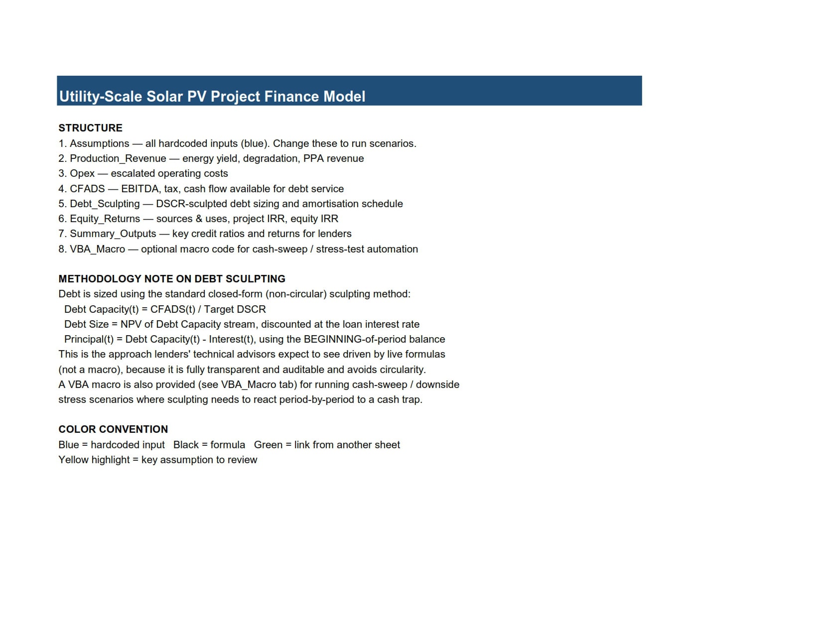
Cover sets out the model’s structure and methodology up front, so a new reader — whether a credit analyst seeing the file for the first time or a sponsor’s own finance team six months after building it — can orient themselves before touching a single cell.
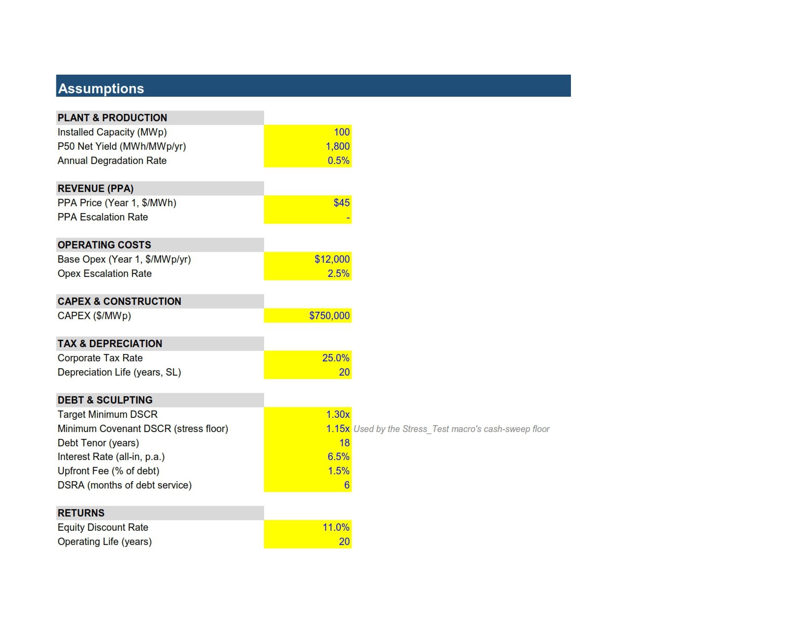
Assumptions holds every hardcoded input in the model, color-coded in blue against a white background so there is never any ambiguity about what is a driver and what is a calculation. Inputs are grouped into plant and production (capacity, yield, degradation), revenue (PPA price and escalation), operating costs, CAPEX, tax and depreciation, debt and sculpting parameters, and return metrics. Centralizing every assumption in one place is not a stylistic preference; it is a structural requirement of a bankable model, because it means a sensitivity run — a lower irradiation case, a higher interest rate, a delayed COD — touches exactly one cell rather than requiring hunting through formulas scattered across multiple tabs.
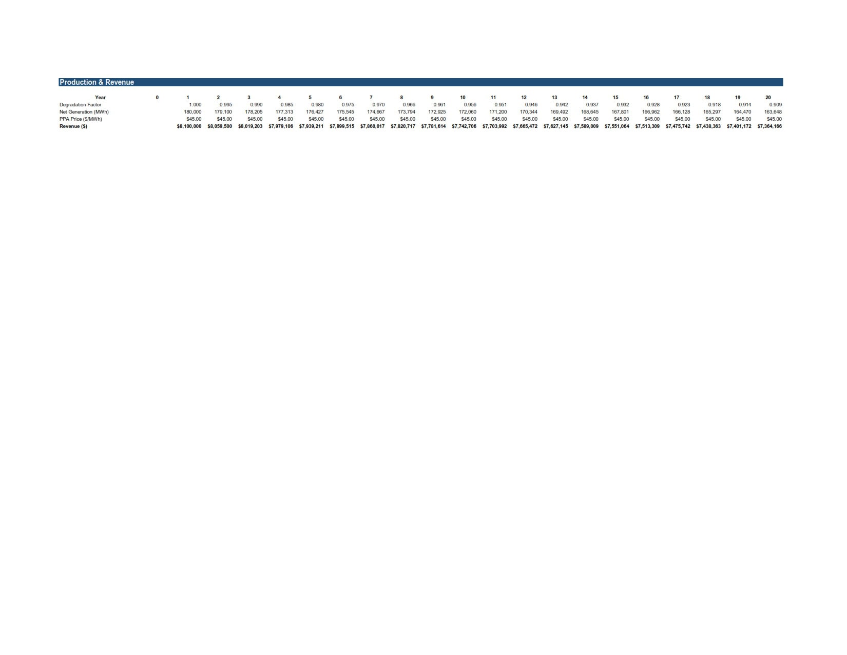
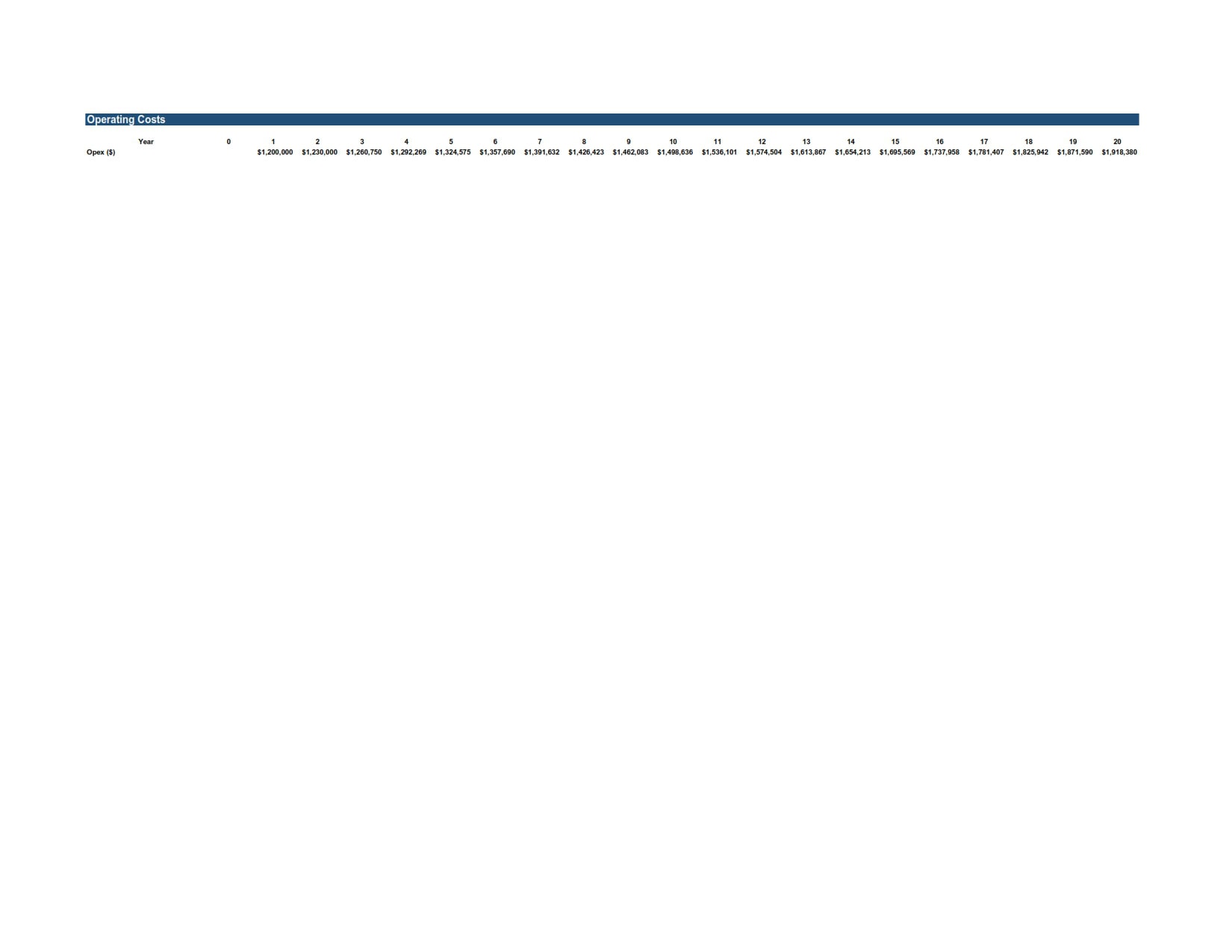
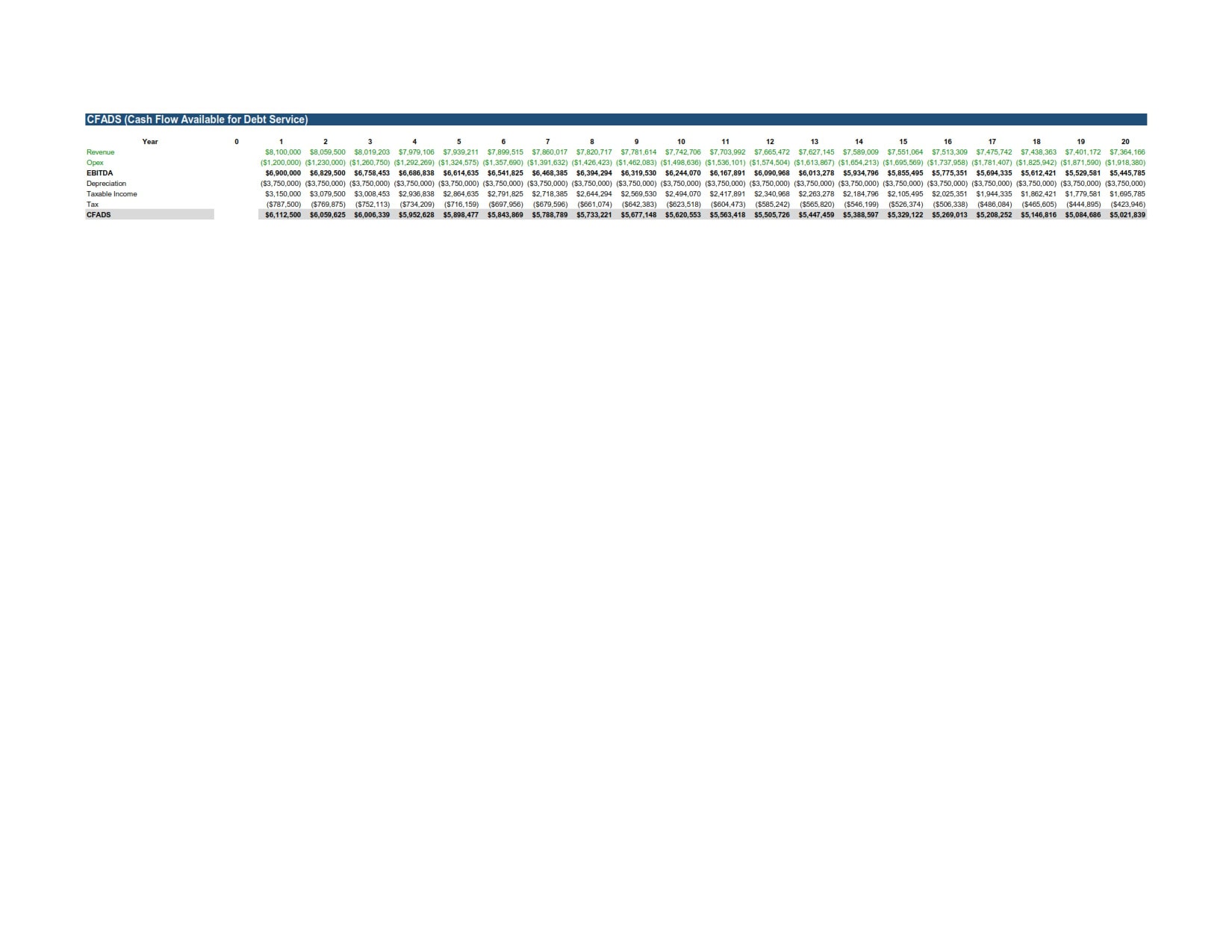
Production_Revenue, Opex, and CFADS form the operational engine of the model. Production_Revenue calculates annual net generation by applying a compounding degradation factor to the plant’s rated yield, then multiplies by an escalating power purchase agreement (PPA) price to arrive at revenue. Opex escalates operating costs at its own independent rate, recognizing that O&M cost inflation and revenue escalation rarely move in lockstep. CFADS — cash flow available for debt service — brings these together into EBITDA, applies straight-line depreciation and corporate tax, and arrives at the single number the entire debt-sizing exercise depends on.
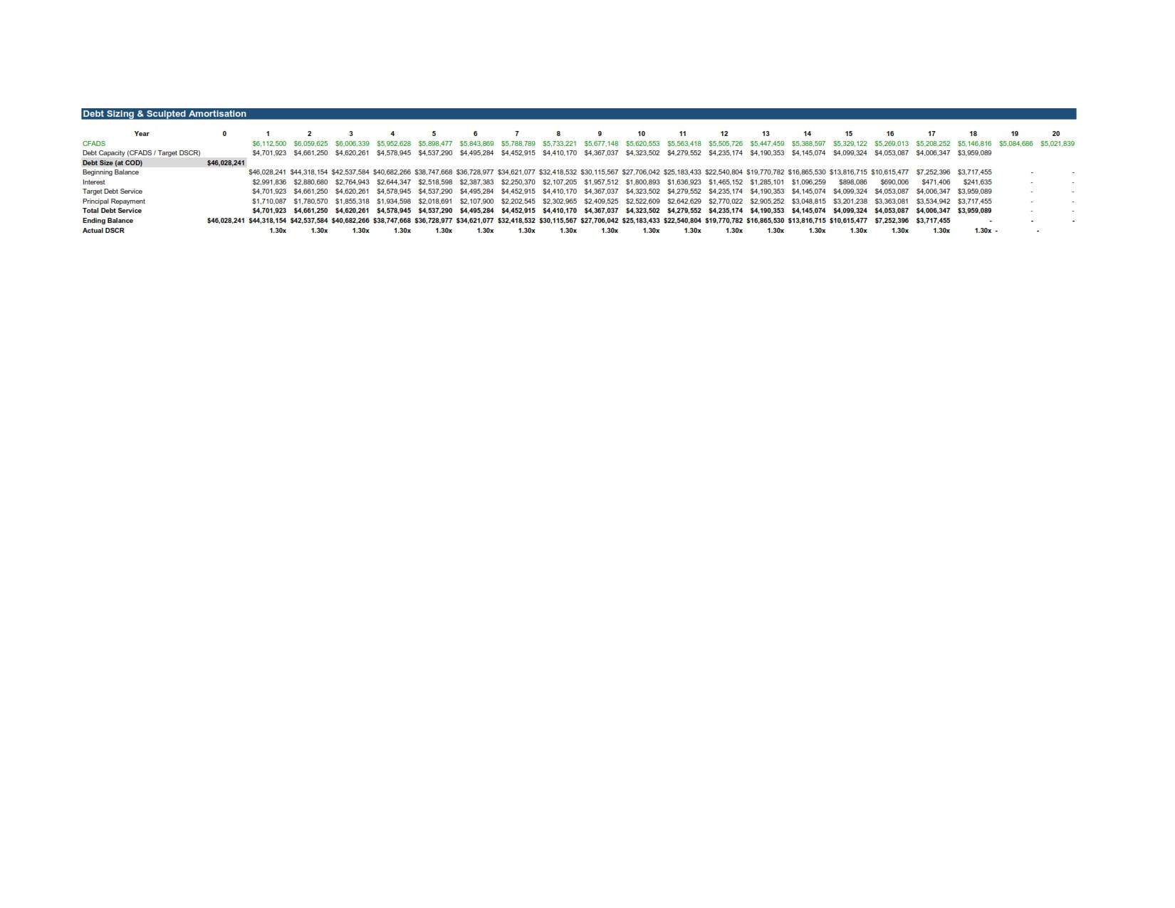
Debt_Sculpting is the heart of the model and the piece that required the most careful engineering. Rather than using a circular reference — a common but fragile approach where interest depends on the balance, which depends on the repayment, which depends on the interest — the model uses a closed-form net present value calculation. The annual “debt capacity” for each year of the loan tenor is defined as CFADS divided by the target minimum DSCR. The total debt size is then simply the net present value of that capacity stream, discounted at the loan’s own interest rate. This works because of a basic identity of loan mathematics: if a loan is repaid using a stream of payments and the interest in every period is calculated on the loan’s own beginning balance, then the present value of that payment stream, discounted at the loan’s rate, exactly equals the original principal — provided the loan fully amortizes to zero. Because the model already guarantees full amortization by construction, this NPV shortcut sizes the debt correctly without ever setting up a circular reference. From there, the model rolls the schedule forward year by year: each year’s beginning balance carries over from the prior year’s ending balance, interest is calculated on that beginning balance, and principal is calculated as the difference between the DSCR-implied debt service and interest, subject to sensible floors and caps. A safeguard in the final year of the tenor forces the balance to zero exactly, cleaning up the last cent of floating-point rounding that would otherwise leave an immaterial residual balance.
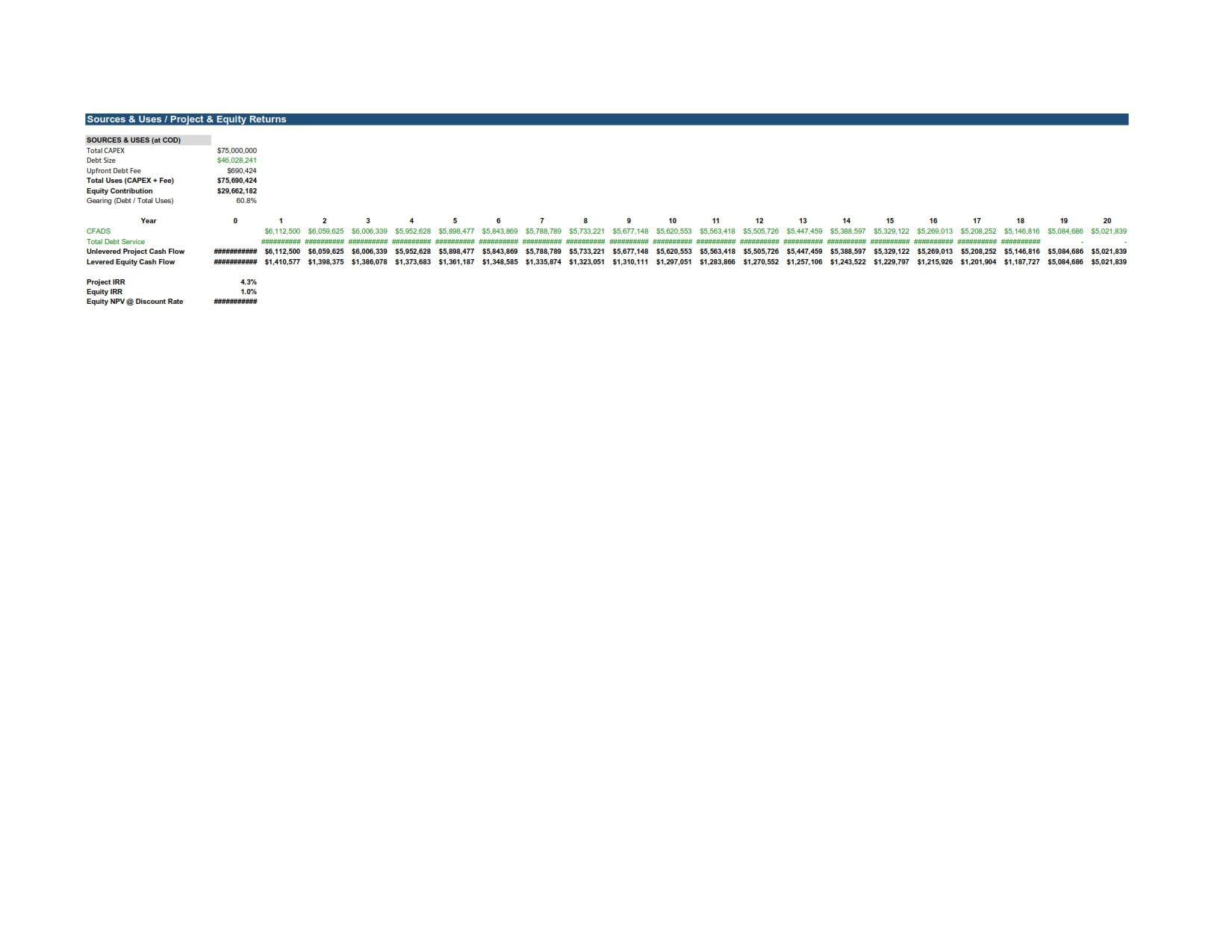
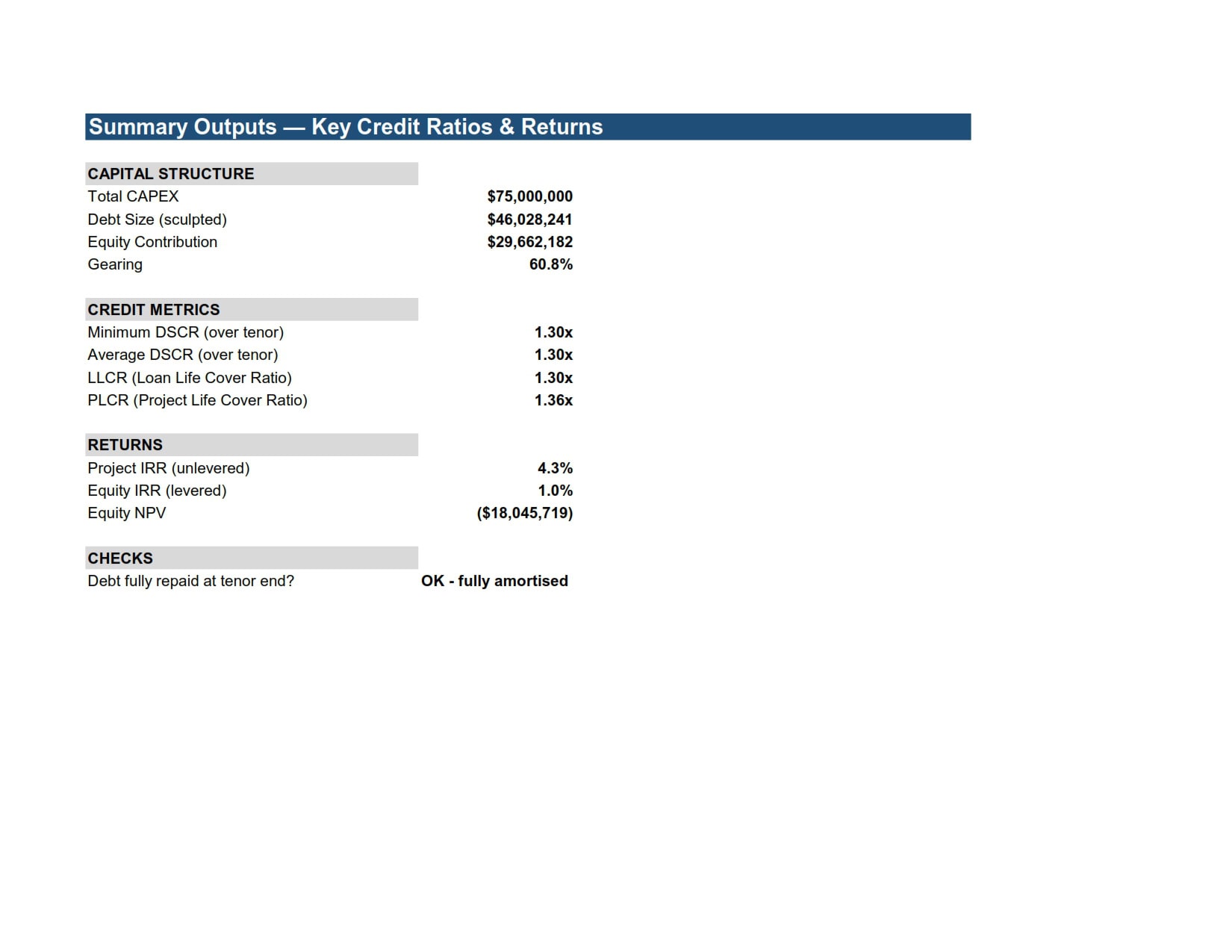
Equity_Returns builds the sources and uses of funds, calculates gearing, and produces both the unlevered project internal rate of return (IRR) and the levered equity IRR, along with an equity net present value at the sponsor’s required discount rate. Summary_Outputs distills everything into the ratios a credit committee actually asks for: minimum and average DSCR across the tenor, the loan life cover ratio (LLCR), the project life cover ratio (PLCR), gearing, and both return metrics, alongside an automated check confirming the debt fully amortizes as designed.
The Stress-Testing Layer
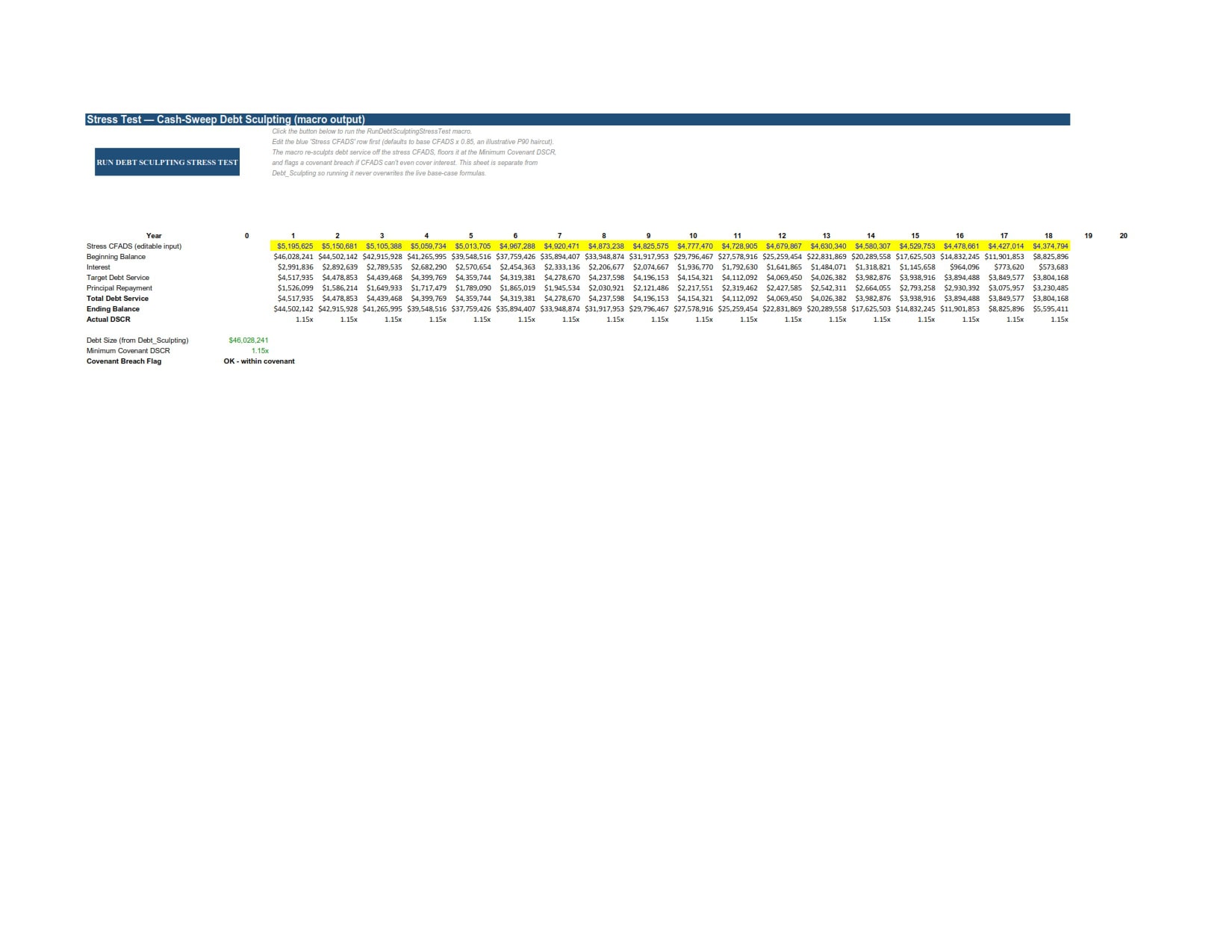
Beyond the base case, the model includes a Stress_Test sheet purpose-built for downside scenario analysis — the kind of exercise a lender’s technical advisor runs to understand what happens if actual production comes in at a P90 (90% probability of exceedance) level rather than the P50 case used for base-case sizing. This sheet is deliberately isolated from the live base-case formulas on the Debt_Sculpting tab, so that running a stress scenario can never accidentally overwrite or corrupt the underlying model that the debt was actually sized against. A dedicated “Minimum Covenant DSCR” assumption — distinct from the target DSCR used for sizing — lets the model distinguish between the DSCR a lender wants to see in the base case and the lower threshold that would actually trigger a covenant breach in a downside scenario.
Running the stress case is intended to be a one-click exercise: an activation button sits directly on the Stress_Test sheet, linked to a documented VBA macro that re-sculpts debt service against a stressed CFADS input, applies the covenant floor, and flags clearly whether the downside case would breach the minimum covenant DSCR in any year of the loan tenor. The macro and its activation are supplied with explicit step-by-step setup instructions on a dedicated tab, since macro-enabled files require a short one-time activation step in Excel before the button becomes live.
Why This Approach Is Considered Bankable
A model earns the description “bankable” not because of its complexity but because of its transparency. Every hardcoded number is visibly an input rather than buried inside a formula. Every credit metric a lender needs — DSCR, LLCR, PLCR — is calculated automatically and can be traced back to its components in seconds. The debt sizing methodology avoids circular references entirely, which matters enormously in practice: circular models are fragile, prone to iterative-calculation settings being disabled by a reviewer who doesn’t realize they need to be on, and difficult for a third party to audit quickly under time pressure. A closed-form NPV-based sculpting approach sidesteps all of that while still producing exactly the DSCR-sculpted repayment profile that project finance lenders expect to see.
Intended Use and Limitations
This model is best understood as a robust, extensible template rather than a finished deal-specific instrument. The illustrative default assumptions — a 100 MWp plant, a flat PPA price, a 65% all-in interest rate margin, and so on — are placeholders meant to demonstrate the mechanics clearly rather than to represent any particular jurisdiction, technology vendor, or offtake structure. Before use in an actual transaction, the tax and depreciation treatment should be reviewed against the specific jurisdiction’s rules (the current build uses a simplified straight-line depreciation approach and excludes the interest tax shield from the tax calculation to preserve the non-circular structure), and the operating assumptions should be replaced with project-specific engineering and market data. Users extending the model for a real transaction may also want to introduce semi-annual periodicity to match typical loan payment conventions, a debt service reserve account cash flow line, and a full three-statement balance sheet check, none of which were required for the core sculpting mechanics this build demonstrates but which a live financing process would typically expect.
Similar ProductsOther customers were also interested in...



 eFinancialModels
Electric Vehicle (EV) Charging Station Financial M...
With this comprehensive 5- or 10-year monthly tool, investors can assess the viability of setting up... Read more

Financial Model for Mobile App | Mobile App Busine...
The Mobile App Financial Plan Template in Excel allows you to develop financial projections when lau... Read more

 HenrySheykin
Food Truck Financial Model Excel Template
The Food Truck Financial Model helps entrepreneurs, founders, business owners, consultants, and anal... Read more

Green Hydrogen Production from Wind Energy Financi...
The Green Hydrogen from Wind Financial Model aims to comprehensively forecast a horizon of 40 years ... Read more

Simple Mutual Non-Disclosure Agreement Template
Protect your business secrets with ease using our Simple Mutual Non-Disclosure Agreement Template. S... Read more

Solar Energy Financial Model
The Solar Energy Financial Model Spreadsheet Template in Excel assists you in preparing a sophistica... Read more

 Peter Graf
The Customer-Centric Financial Model for Restauran...
Starting a restaurant without a financial plan is like driving a car blindfolded. You wouldn´t do i... Read more
You must log in to submit a review.