
0 ITEMS

CO₂ Liquefaction, Shipping & Storage Terminal Financial Model | 30-Year Excel Project Finance Template
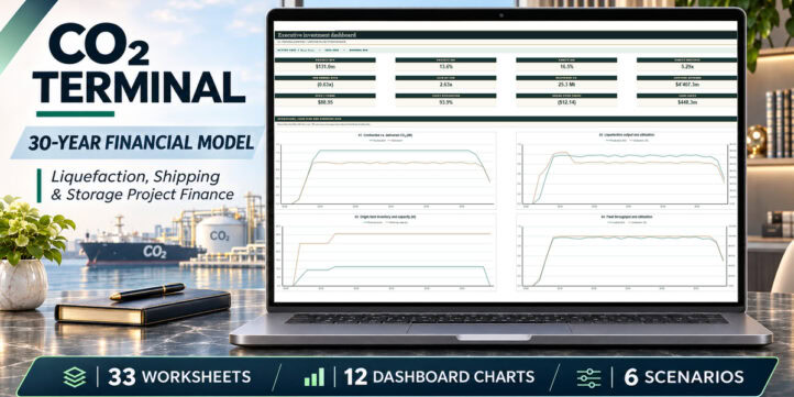
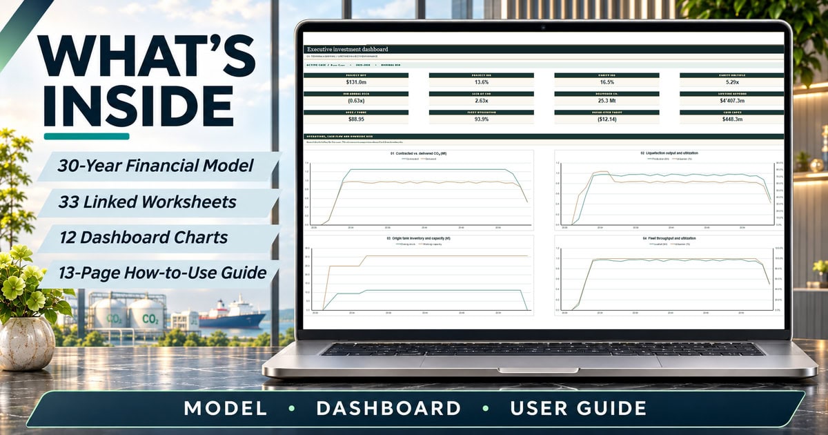
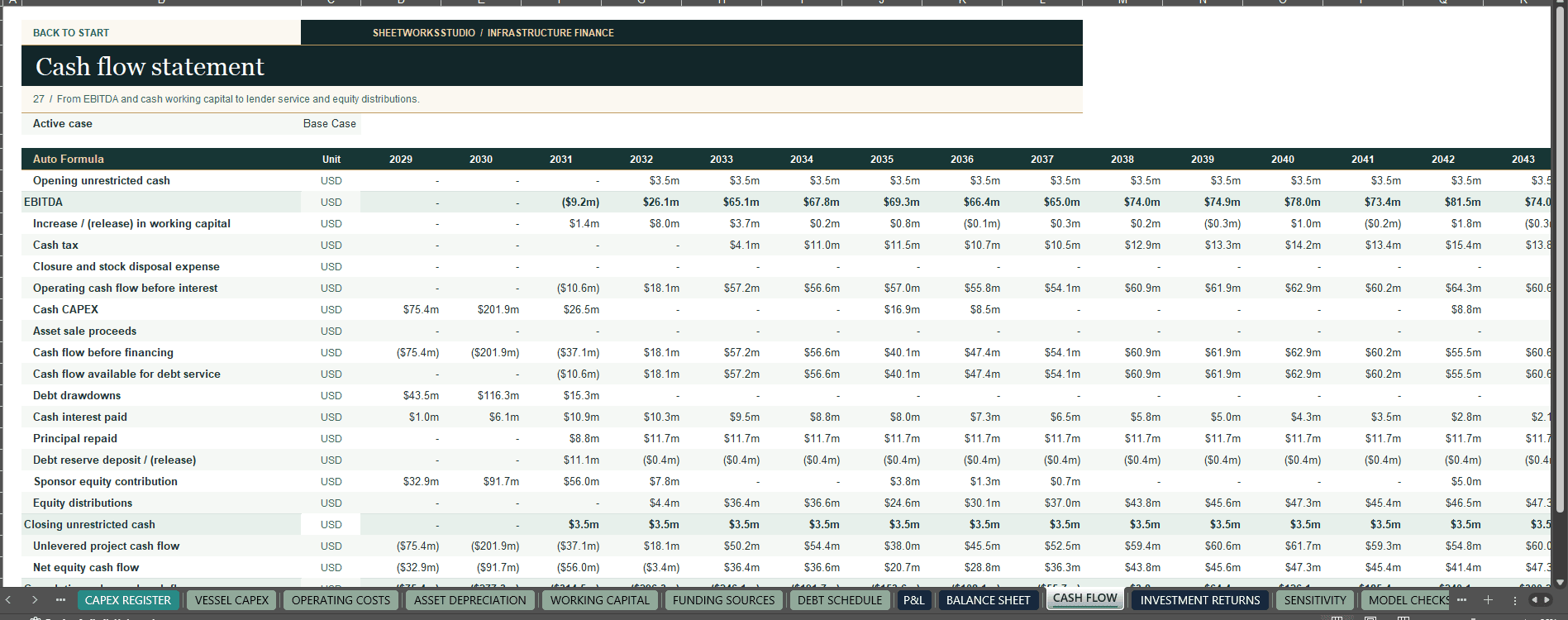
Evaluate a CO₂ liquefaction, shipping or terminal storage project over 30 years. Trace contracted tonnes through processing, tanks, vessels and terminal capacity, then review the impact on revenue, cash flow, debt coverage and investment returns. Includes 360 monthly periods, 30 annual summaries, six selectable scenarios, 12 dashboard charts and a 13-page English user guide.
CO₂ Liquefaction, Shipping & Storage Terminal Financial Model
30-Year Excel Project Finance Template for CO₂ Infrastructure
360 monthly periods · 30 annual summaries · 33 worksheets · 6 selectable scenarios · 12 dashboard charts
How many contracted tonnes can your infrastructure actually deliver, and what does that mean for revenue, funding and debt coverage?
A terminal can have contracted demand but insufficient available supply. A liquefaction plant can produce enough CO₂ while tank space, berth slots or vessel availability limit deliveries. And a project with a positive net present value can still face a cash shortfall or breach its modeled debt coverage threshold in a particular month.
The CO₂ Liquefaction, Shipping & Storage Terminal Financial Model puts those questions on one timeline. It connects contracted demand and physical throughput to tariffs, operating costs, capital investment, financing and investment returns. Use the monthly schedules to locate the bottleneck or funding pressure, then use the annual summaries and executive dashboard to see what it means for the project over 30 years.
🏗️ Choose the infrastructure you want to evaluate
The workbook supports five project configurations. Start by defining which services and assets belong inside your project before entering tariffs, capital costs or fleet assumptions.
Configuration What to examine Liquefaction only CO₂ intake, pretreatment, liquefaction output and the cost of delivering the liquefaction service. Export terminal Origin-side tank capacity, handling and loading, and how export constraints affect throughput. Integrated shipping The interaction between liquefaction, origin storage, vessel operations and receiving-side delivery. Import terminal Receiving, unloading and delivery constraints without treating the entire upstream chain as owned infrastructure. Multi-customer network How different customer ramp-up schedules, contract volumes and tariff classes interact with shared capacity.
The PROJECT CONFIG sheet shows which stages and billing components are enabled in each configuration. Where the model includes a partner buffer, treat it as a modeled interface, not as an asset owned by the project.
When shipping is in scope, choose owned vessels, chartered vessels or third-party shipping charged per voyage. Compare the effect on fleet investment and operating costs as well as the number of tonnes the fleet can move. A lower upfront fleet investment does not necessarily result in a lower lifetime cost.
⚙️ Follow the tonnes from supply to delivery
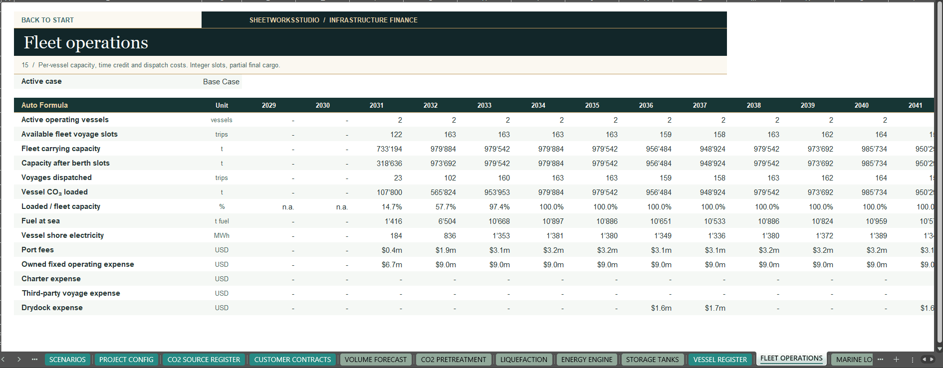
The workbook distinguishes offered supply, contracted demand, processed CO₂, stored inventory, shipped tonnes, unloaded tonnes and delivered tonnes. These quantities do not have to match in a given month. The physical schedules help explain the difference.
- CO₂ supply and pretreatment. Set the timing, ramp-up, purity, availability and pretreatment losses for source inputs. Review how much offered supply is admitted to the process and compare it with contracted demand.
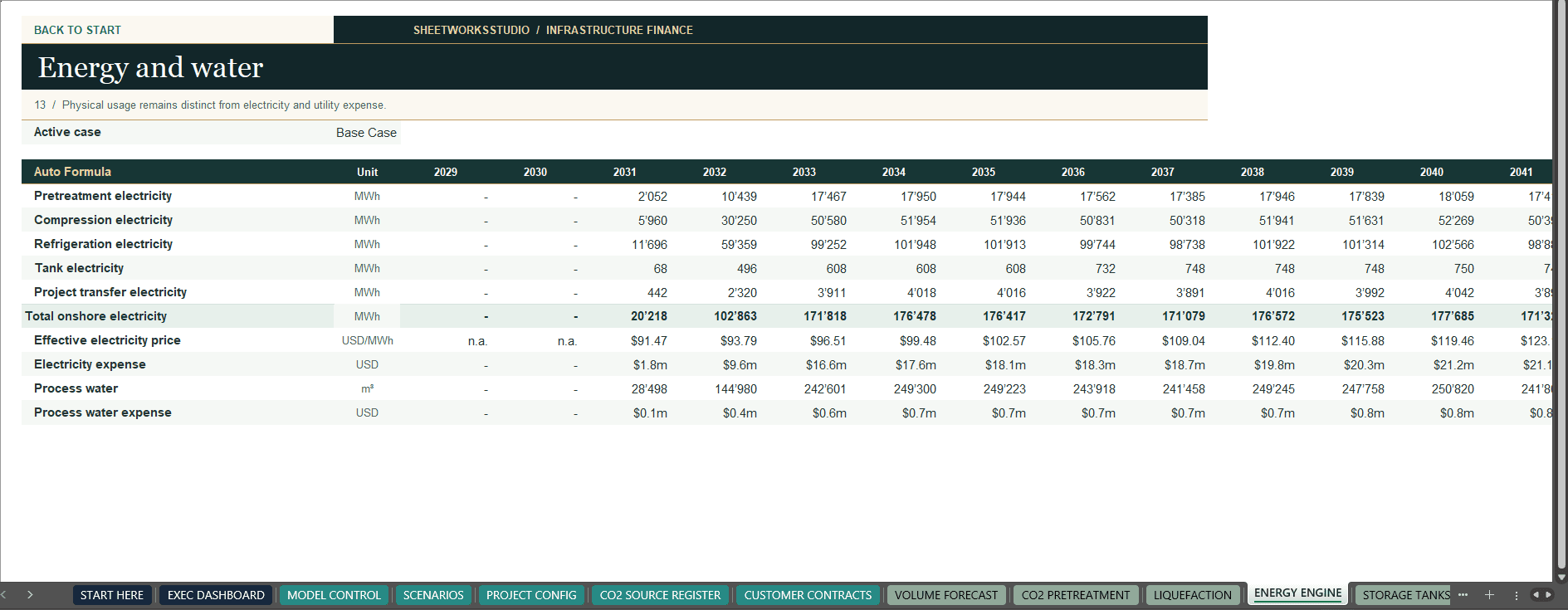
- Liquefaction and energy. Follow usable capacity, mechanical availability and recovery through to liquefaction output. Review electricity intensity and standing tank loads under the selected power pricing assumptions.
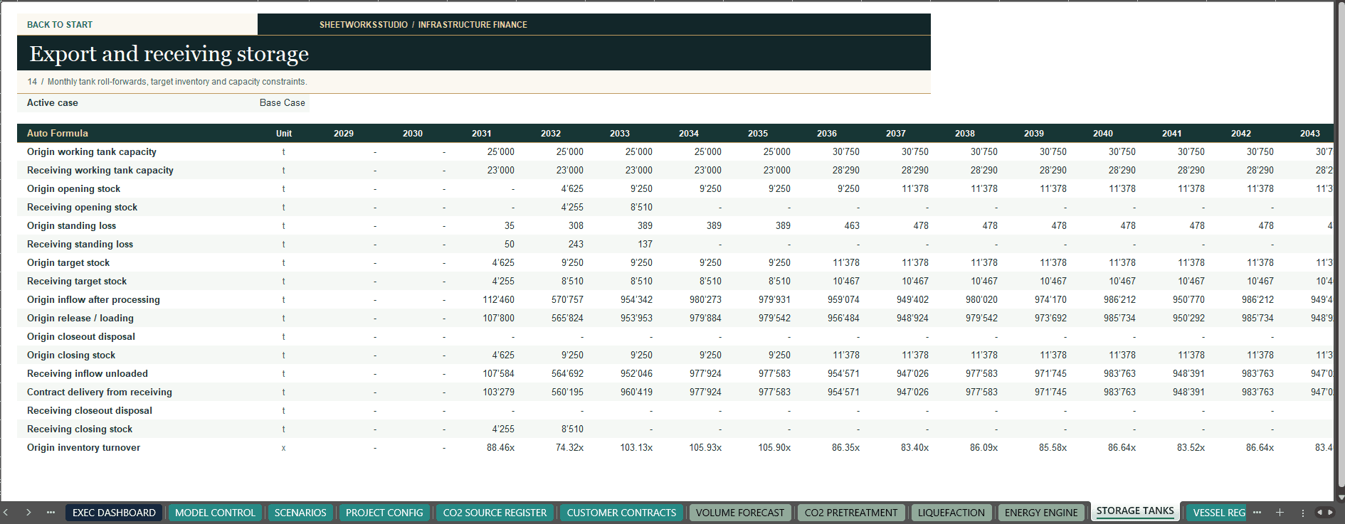
- Tank inventory. Trace opening stock, additions, withdrawals, losses and closing stock. Compare the buffer with usable tank capacity and review whether storage is constraining throughput.
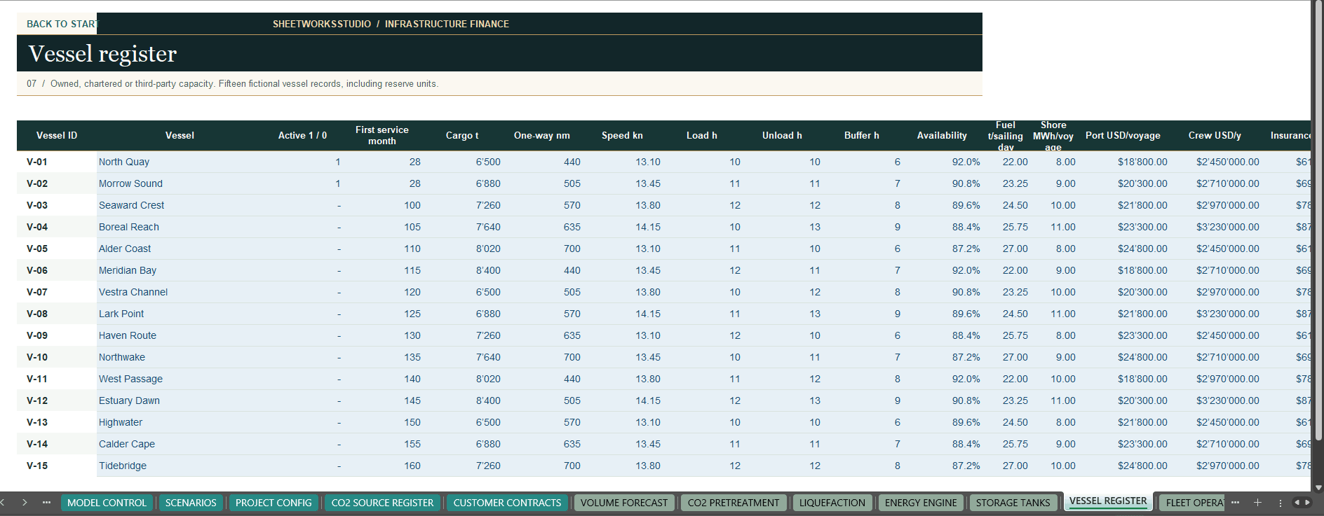
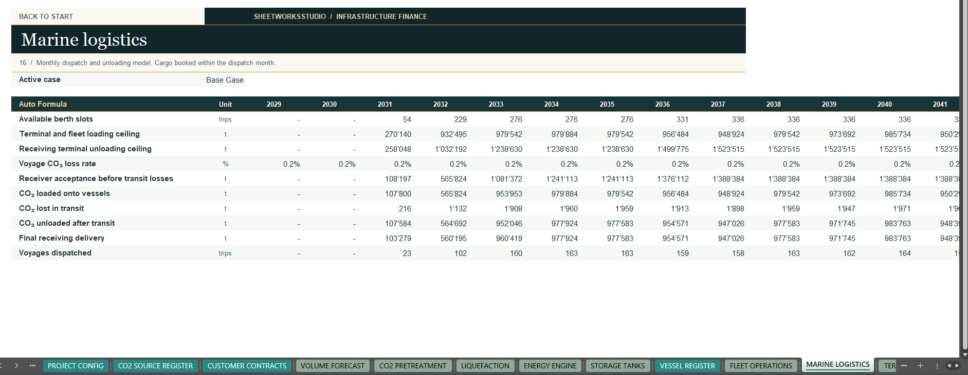
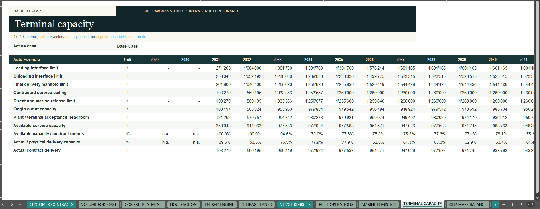
- Vessel and terminal operations. Review payload, voyage distance, speed, port time, available trips, berth slots and loading or unloading limits. A vessel’s nominal payload alone does not determine monthly fleet throughput.
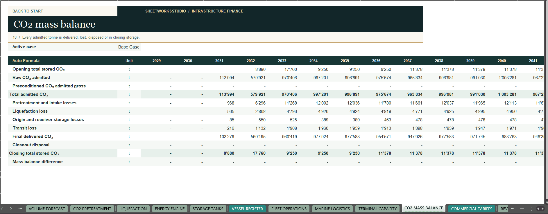
- Mass balance. Trace movements and losses across the modeled chain. Use the reconciliation checks to distinguish a physical shortfall from an inconsistency in the model.
A practical diagnostic: If contracted volumes rise but deliveries do not, compare available supply, liquefaction output, tank stock and vessel or berth capacity in that order. Raising the tariff does not remove a physical bottleneck. Increasing liquefaction capacity may not help if shipping is already limiting deliveries.
Shipping is modeled at monthly planning level. The workbook uses whole voyage slots and approximates within-month handling and arrival timing. It is not a vessel dispatch or berth scheduling system.
📋 Connect contracts and tariffs to invoices and cash receipts
The commercial schedules separate what a customer contracts for, what the project delivers and what the project bills and collects. That distinction matters when customers ramp up at different speeds or when available capacity falls short of contracted demand.
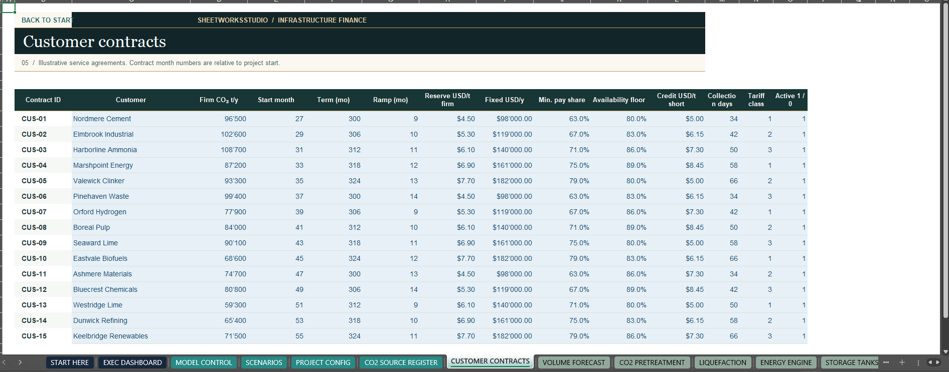
- Enter firm annual tonnes, contract start and term, ramp-up, collection days and tariff class in CUSTOMER CONTRACTS.
- Use COMMERCIAL TARIFFS to review per-tonne rates for liquefaction, origin handling, shipping and receiving services where applicable.
- Review delivered-service revenue separately from reservation fees, fixed availability charges and eligible ship-or-pay charges.
- Test how minimum payment terms, availability thresholds and shortfall credits affect billing under the workbook’s modeled rules.
- Follow invoiced amounts into receivables, collections and working capital. A month with higher billed revenue is not necessarily a month with higher cash receipts.
Ship-or-pay treatment depends on eligible unused capacity that the project made available under the modeled rules. It is not an assumption that all undelivered contracted tonnes are automatically billable. Review your own contracts before applying the model’s commercial logic to a real project.
💰 Review capital spending, debt and sponsor funding
Follow onshore and vessel capital expenditure, depreciation and working capital through the linked profit and loss statement, balance sheet and cash flow statement. Review expenditure during construction, commissioning and expansion separately from the cost of ongoing operations.
The financing schedules cover:
- Debt drawdowns based on the scenario-adjusted debt share of eligible initial CAPEX.
- Interest and principal repayment, with level principal beginning at commercial operation under the modeled terms.
- Debt service reserve account (DSRA) funding and release, with the reserve target based on upcoming scheduled debt service.
- Sponsor equity and liquidity support, including an optional cap on total sponsor equity.
- Distributions and debt coverage, including the ability to block distributions when monthly DSCR falls below the modeled threshold.
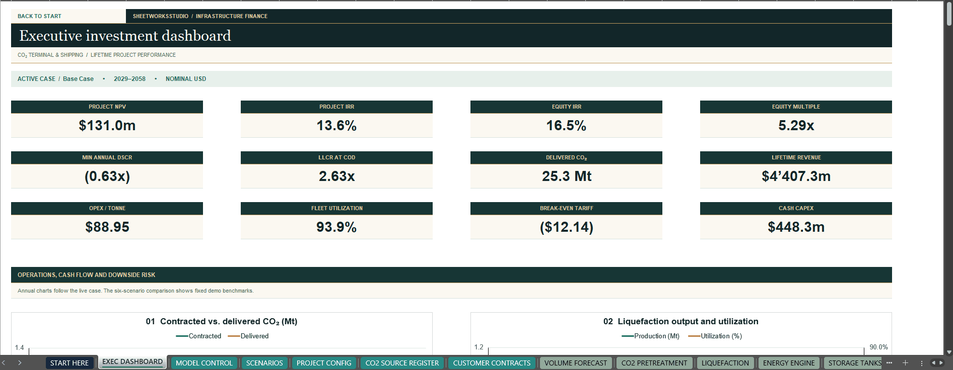
Profitability, liquidity and debt coverage answer different questions. A project can show a positive NPV while still failing its DSCR threshold in certain months. The fictional Base Case illustrates this distinction. The model reports commercial coverage warnings separately from reconciliation failures, so a debt coverage warning is not, by itself, a spreadsheet error.
A negative cash balance can reveal an unfunded requirement. It should not be read as an automatic new debt draw or a commitment from a lender.
🔄 Test six scenarios, one live case at a time
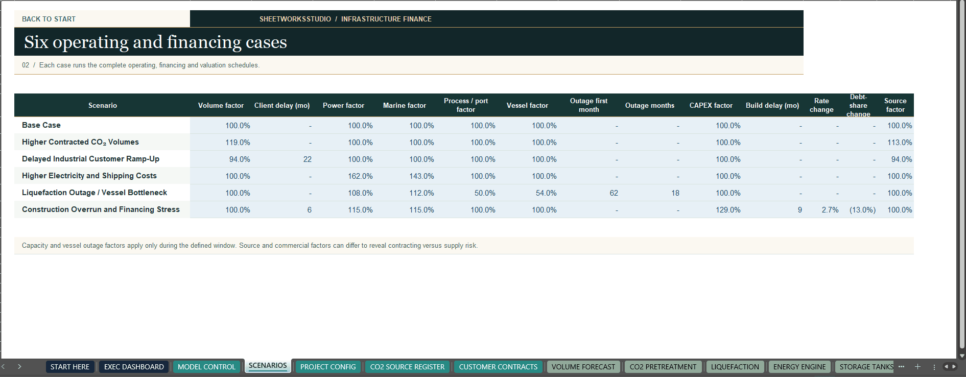
Scenario What it helps you investigate 1. Base Case Establish the reference operating, commercial and financing assumptions. 2. Higher Contracted CO₂ Volumes Test whether more contracted demand translates into higher deliveries or exposes a capacity constraint. 3. Delayed Industrial Customer Ramp-Up Examine the effect of later customer demand on utilisation, revenue and funding needs. 4. Higher Electricity and Shipping Costs Review how higher energy and marine costs affect operating economics and cash flow. 5. Liquefaction Outage / Vessel Bottleneck Test reduced process, terminal or fleet availability during a defined outage window. 6. Construction Overrun and Financing Stress Examine the combined effect of higher CAPEX, delayed completion and changed financing assumptions.
What updates live: The scenario selected in MODEL CONTROL drives the active operating, financial and valuation schedules. For your current results, read the Active case column in INVESTMENT RETURNS.
What stays fixed: The six demo comparison columns and the dashboard’s Demo Scenario Benchmarks chart show fixed illustrative results. They do not update when you edit the model. To compare cases using your own project assumptions, select them one at a time and record each live result separately.
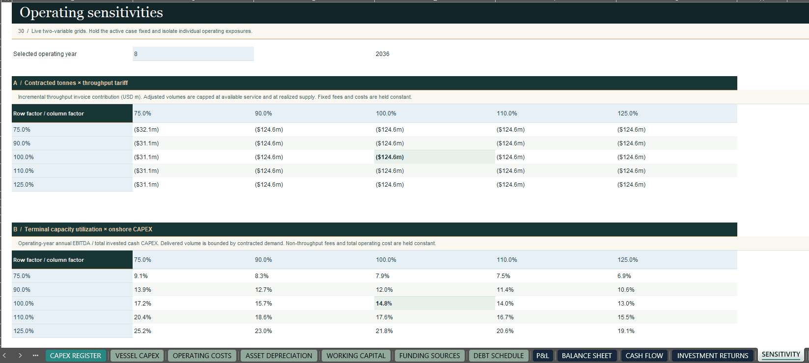
Three additional sensitivity grids let you examine selected relationships involving contracted tonnes and tariffs, terminal utilisation and onshore CAPEX, and fleet availability and operating costs. They are operating diagnostics for a selected year, not separate 30-year project NPV recalculations for every input combination.
📊 Read the dashboard, then trace the result
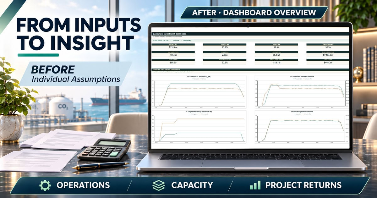
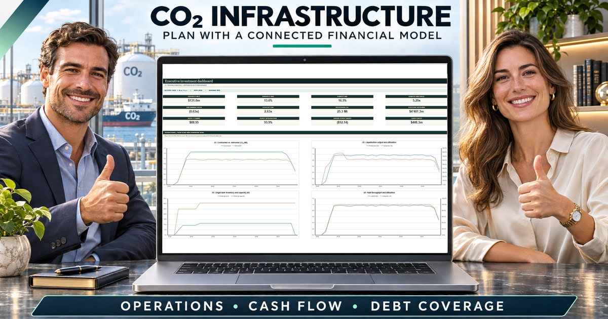
The executive dashboard brings together project NPV, project IRR, equity IRR, equity multiple, delivered CO₂, lifetime revenue, operating cost per delivered tonne, fleet utilisation, DSCR and LLCR. Use it to identify what changed, then open the schedule behind the number to understand why.
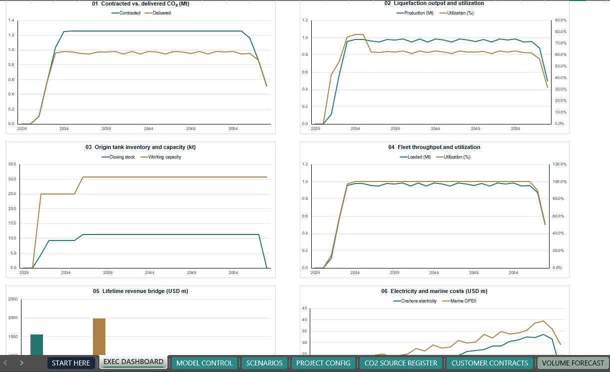
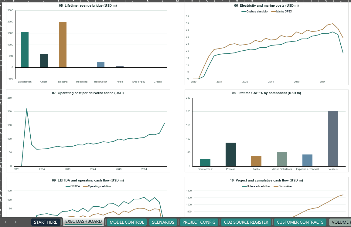
Dashboard view What the charts show Throughput and capacity Contracted versus delivered CO₂, liquefaction output and utilisation, origin tank inventory and capacity, and fleet throughput and utilisation. Operating economics Lifetime revenue by component, electricity and marine costs, and operating cost per delivered tonne. Investment and credit CAPEX by component, EBITDA and operating cash flow, project and cumulative cash flow, and closing debt alongside annual DSCR. Illustrative benchmarks A fixed comparison of project NPV and equity IRR across the six demo cases.
Use project returns to examine the economics of the infrastructure and equity returns to examine the timing of sponsor contributions and distributions. Read DSCR and LLCR alongside those returns. They describe debt coverage rather than the profitability of the investment. The detailed checks include physical reconciliation, debt and reserve roll-forwards, balance sheet balance and cash flow reconciliation.
✏️ Build your own case from the included example
The workbook is prefilled with fictional, editable example data. Use the example to understand how the schedules connect, then replace the designated inputs with your project assumptions. The shipped Base Case uses nominal USD and starts in January 2029. The start year is editable in MODEL CONTROL, cell C8.
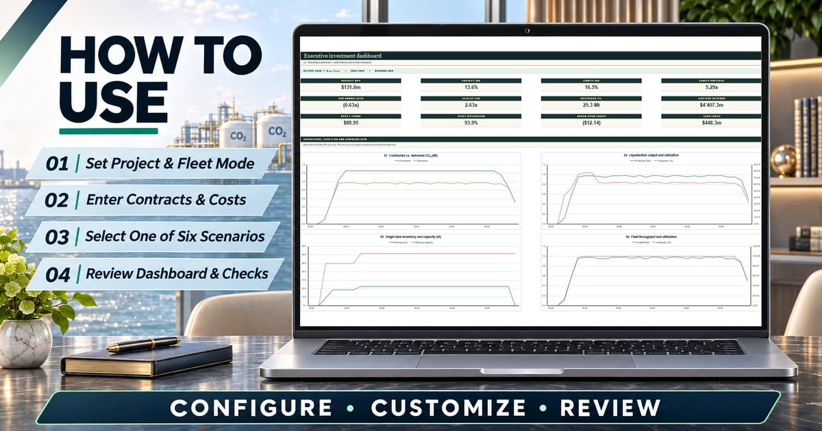
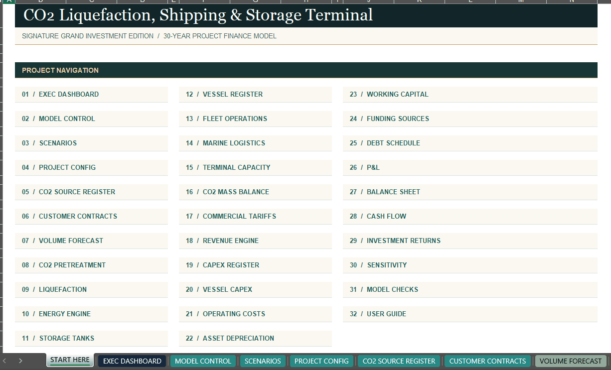
- Set the project scope. Open START HERE, then select the calendar, project configuration, fleet mode and live scenario.
- Enter commercial and operating inputs. Update source availability, customer contracts, tariffs, process capacity, tank assumptions and marine inputs.
- Set investment and funding assumptions. Review the construction and commissioning schedule, CAPEX, debt terms, minimum cash and sponsor support.
- Check the physical results first. Compare contracted and delivered tonnes and review any capacity constraint or inventory imbalance.
- Review the financial results. Use the active case, financial statements and model checks to interpret liquidity, debt coverage and investment returns.
The included guide identifies the main control cells, maps the worksheets and shows how to investigate results rather than simply reading the dashboard.
📦 What you receive
One ZIP download containing:
- CO₂ Liquefaction, Shipping & Storage Terminal 30-Year Financial Model (.xlsx)
- 13-page English How-to-Use Guide in A4 PDF format (.pdf)
The full guide is also available as a separate free download to review the model’s structure and workflow before purchasing. This is a digital product. No physical item or spreadsheet software is included.
💻 Format, compatibility and calculation time
The workbook and guide are in English. The workbook is macro-free and has no external data connections. Microsoft Excel Desktop with Automatic Calculation enabled is recommended for the intended workflow.
The workbook has been opened and checked in LibreOffice. Full recalculation in Microsoft Excel Desktop and compatibility with Google Sheets have not been verified. Because the workbook contains 360 months of linked operating and financial schedules, opening or recalculation may take longer than with a basic spreadsheet. Allow calculation to finish before reading results or changing the scenario again.
Who this model is for
Designed for infrastructure analysts, project developers, finance teams, consultants and investment professionals evaluating CO₂ terminal, liquefaction or shipping projects. It is particularly useful when you need to explain not only whether the project appears viable under a set of assumptions, but which physical, commercial or financing assumption drives that result.
Scope and interpretation
Terminal storage means above-ground tank and buffer storage within the modeled logistics chain. The workbook is not a geological injection or subsurface storage model. Handling, shipping or delivery of CO₂ does not demonstrate permanent sequestration.
This is an independent, unofficial financial planning template. Included assumptions and results are illustrative, not engineering specifications, supplier quotations, bank-approved forecasts, investment recommendations or guaranteed outcomes. Validate technical assumptions, contracts, tariffs and financing terms against your own project before relying on the results.
SheetworksStudio
Similar ProductsOther customers were also interested in...



 eFinancialModels
Electric Vehicle (EV) Charging Station Financial M...
With this comprehensive 5- or 10-year monthly tool, investors can assess the viability of setting up... Read more

Financial Model for Mobile App | Mobile App Busine...
The Mobile App Financial Plan Template in Excel allows you to develop financial projections when lau... Read more

 HenrySheykin
Food Truck Financial Model Excel Template
The Food Truck Financial Model helps entrepreneurs, founders, business owners, consultants, and anal... Read more

Green Hydrogen Production from Wind Energy Financi...
The Green Hydrogen from Wind Financial Model aims to comprehensively forecast a horizon of 40 years ... Read more

Simple Mutual Non-Disclosure Agreement Template
Protect your business secrets with ease using our Simple Mutual Non-Disclosure Agreement Template. S... Read more

Solar Energy Financial Model
The Solar Energy Financial Model Spreadsheet Template in Excel assists you in preparing a sophistica... Read more

 Peter Graf
The Customer-Centric Financial Model for Restauran...
Starting a restaurant without a financial plan is like driving a car blindfolded. You wouldn´t do i... Read more
You must log in to submit a review.