0 ITEMS

Excel Rounding to 2 Decimal Places: ROUND vs Format
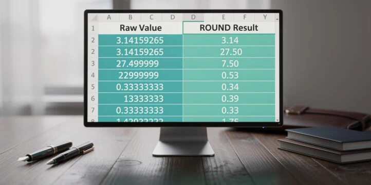
To show only 2 decimal places in Excel, you have two distinct options: the ROUND function changes the actual stored value, while Format Cells changes only what you see on screen.
Key Takeaways
=ROUND(A1,2)is the correct formula when you need the underlying number to be mathematically rounded to 2 decimal places, not just displayed that way.- Format Cells (Ctrl+1) changes the visual display only; the stored value stays at full precision, which can cause silent calculation errors downstream.
- ROUNDUP always rounds away from zero, ROUNDDOWN always rounds toward zero, and MROUND rounds to the nearest specified multiple — each serves a different financial use case.
- Rounding errors compound in formula chains: rounding a 6-decimal intermediate result before passing it to a SUM can shift a final total by several cents across thousands of rows.
- The
ROUNDfunction accepts a second argument (num_digits) of 2 to target 2 decimal places; negative values round to tens, hundreds, and so on. - Excel’s “Precision as Displayed” setting permanently overwrites stored values to match the visual format — use it only when you fully understand the consequences.
- For professional financial models, round at the final output stage, not mid-calculation, to preserve accuracy throughout the formula chain.
Format vs. Function: The Distinction That Matters
The single most important concept in Excel decimal control is that formatting and rounding are not the same thing. Format Cells tells Excel how to display a number; the ROUND function tells Excel to store a different number.
Here is why this matters in practice. Suppose cell A1 contains 10.2567. If you format A1 to show 2 decimal places, the cell displays 10.26, but the value Excel uses in every downstream formula is still 10.2567. If you instead enter =ROUND(A1,2) in cell B1, B1 stores and uses 10.26 in every subsequent calculation.
According to Microsoft’s official documentation, the ROUND function rounds a number to a specified number of digits, using standard half-up rounding.
Format Cells, by contrast, is purely cosmetic.
When to use each:
- Use
ROUNDwhen the rounded value feeds into further calculations (invoices, tax lines, financial statement subtotals). - Use Format Cells when you only need clean visual presentation and all downstream formulas reference the original full-precision value.
Format Cells and ROUND look identical on screen but behave completely differently in calculations.
Method 1: The ROUND Function
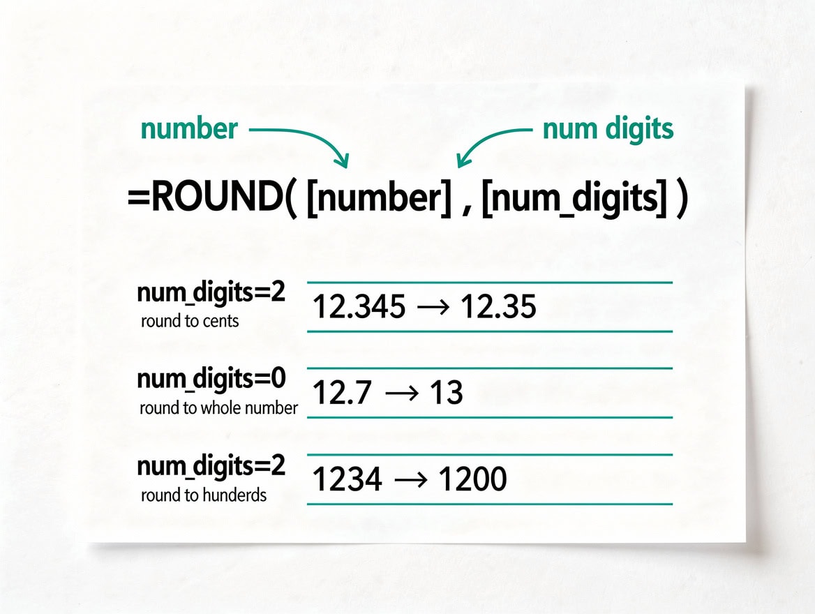
The ROUND function is the standard mathematical approach to limiting decimal places in Excel. Its syntax is =ROUND(number, num_digits), where number is the value or cell reference and num_digits is the decimal place target.
Syntax breakdown:
number: the value to round (can be a cell reference, a formula result, or a literal number)num_digits: 2 for two decimal places; 0 for whole numbers; -1 to round to the nearest 10
Step-by-step:
- Click the cell where you want the rounded result.
- Type
=ROUND( - Click the source cell (e.g., A1) or type the number.
- Type
,2)to set 2 decimal places. - Press Enter.
Excel applies standard half-up rounding: values at or above the midpoint round up, values below round down. The ROUND function accepts a num_digits argument ranging from negative numbers up to 15 significant digits of precision.
This gives you fine-grained control over every rounding scenario in a financial model.
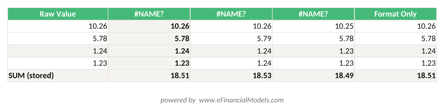
=ROUND(A2,2) stores the mathematically rounded value; columns C and D show directional rounding alternatives.
Method 2: Format Cells for Visual Display
Format Cells changes how a number looks without altering its stored value. This is the right choice for dashboards, printed reports, and any situation where the raw precision must stay intact for calculations.
Step-by-step (keyboard method):
- Select the cell or range you want to format.
- Press Ctrl+1 to open the Format Cells dialog.
- Click the Number tab.
- Select Number from the Category list.
- Set Decimal places to 2.
- Click OK.
Ribbon shortcut: On the Home tab, use the “Decrease Decimal” button (the icon showing a left-pointing arrow with decimal digits) to reduce displayed decimals one step at a time.
Critical reminder: After applying this format, if A1 displays 10.26 but stores 10.2567, then =A1*100 returns 1025.67, not 1026.00. The display and the math diverge silently. Excel stores numbers with up to 15 significant digits of precision.
This means the gap between a formatted display value and its stored counterpart can be substantial across many decimal places.
Ctrl+1 opens Format Cells instantly; set Decimal places to 2 for visual-only formatting.
ROUNDUP, ROUNDDOWN, MROUND, and CEILING
Excel provides four additional rounding functions for cases where standard half-up rounding does not fit the business rule. Each function changes the actual stored value, just like ROUND.
- ROUNDUP (
=ROUNDUP(number, num_digits)): always rounds away from zero, regardless of the digit. Use this for conservative cost estimates or tax calculations where you must never understate. - ROUNDDOWN (
=ROUNDDOWN(number, num_digits)): always rounds toward zero. Use this when you must never overstate a value, such as calculating maximum allowable deductions. - MROUND (
=MROUND(number, multiple)): rounds to the nearest specified multiple.=MROUND(A1, 0.05)rounds to the nearest 5 cents, useful for cash-register pricing. - CEILING (
=CEILING(number, significance)): rounds up to the nearest multiple of significance.=CEILING(A1, 0.01)always rounds up to the next cent. - FLOOR (
=FLOOR(number, significance)): rounds down to the nearest multiple of significance.
ROUNDUP and ROUNDDOWN give directional control; MROUND rounds to a specified multiple like 0.05.
Quick Reference: All Rounding Methods Compared
| Function | Syntax | Changes Value? | Direction | Best Use Case |
|---|---|---|---|---|
| ROUND | =ROUND(A1,2) | Yes | Half-up | General financial rounding |
| ROUNDUP | =ROUNDUP(A1,2) | Yes | Always up | Conservative estimates, tax |
| ROUNDDOWN | =ROUNDDOWN(A1,2) | Yes | Always down | Maximum deduction limits |
| MROUND | =MROUND(A1,0.05) | Yes | Nearest multiple | Cash pricing, 5-cent increments |
| CEILING | =CEILING(A1,0.01) | Yes | Always up to multiple | Billing, always-round-up rules |
| FLOOR | =FLOOR(A1,0.01) | Yes | Always down to multiple | Conservative revenue recognition |
| Format Cells | Ctrl+1 | No | Display only | Reports, dashboards |
Worked Numerical Example: Rounding Error in a Formula Chain
This example shows exactly how a formatting-only approach creates a calculation error that the ROUND function prevents.
Scenario: You have three line items on an invoice.
- Item A: 4.3333 (stored value)
- Item B: 2.6667 (stored value)
- Item C: 1.0000 (stored value)
Step 1: Format-only approach
You format all three cells to display 2 decimal places. They show 4.33, 2.67, and 1.00. The SUM formula =A1+A2+A3 returns 8.00 on screen (formatted), but the actual stored result is 4.3333 + 2.6667 + 1.0000 = 8.0000. In this case the totals match, but watch what happens with a different set:
- Item A: 1.2350 displays as 1.24 (rounds up)
- Item B: 1.2350 displays as 1.24 (rounds up)
- Item C: 1.2350 displays as 1.24 (rounds up)
Displayed total: 1.24 + 1.24 + 1.24 = 3.72
Actual SUM: 1.2350 + 1.2350 + 1.2350 = 3.705, which formats to 3.71
Result: the displayed line items sum to 3.72, but the displayed total shows 3.71. This is the classic “cents don’t add up” audit finding.
Step 2: ROUND function approach
Replace each raw value with =ROUND(raw_value, 2). Now each cell stores exactly 1.24. The SUM stores and displays 3.72. The line items and the total are consistent.
Here’s the math:
=ROUND(1.2350, 2) → stores 1.24=ROUND(1.2350, 2) → stores 1.24=ROUND(1.2350, 2) → stores 1.24=SUM(B1:B3) → 3.72 (stored and displayed)
No discrepancy. No audit flag.
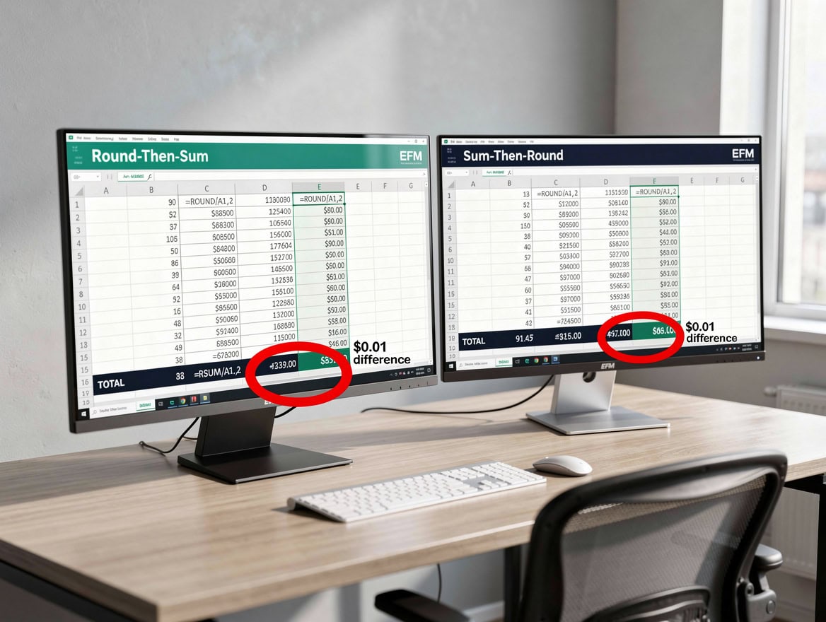
The classic audit finding: formatted line items sum to 3.72 but the total cell shows 3.71.
Applying Decimal Formatting to Entire Columns
Formatting a single cell is straightforward, but financial models often require consistent formatting across hundreds of rows. Excel makes this efficient with a few techniques.
Select an entire column: Click the column letter (e.g., “B”) to select all cells, then press Ctrl+1 and set decimal places to 2. Every cell in that column, including future entries, inherits the format.
Select a named range: If your data lives in a defined table (Insert > Table), format the column once and Excel automatically extends the format to new rows added at the bottom.
Paste Special for format only: Format one cell correctly, copy it (Ctrl+C), select the target range, press Ctrl+Alt+V, choose “Formats”, and click OK. This applies the number format without overwriting values.

Select the entire column letter to apply 2-decimal formatting to all current and future entries at once.
Common Rounding Mistakes and How to Fix Them
Even experienced analysts make these five errors. Each one has a clear fix.
Mistake 1: Relying on Format Cells for financial totals
Fix: Use =ROUND(value, 2) on every input that feeds a SUM or subtotal. Format Cells for display only.
Mistake 2: Rounding intermediate values mid-chain
Fix: Keep full precision through all intermediate calculations. Apply ROUND only to the final output cell. Rounding at each step compounds the error.
Mistake 3: Using ROUNDUP when standard rounding is required
Fix: ROUNDUP always rounds away from zero, so 2.501 and 2.999 both become 2.51 with =ROUNDUP(value,2). Use ROUND unless a specific business rule requires directional rounding.
Mistake 4: Enabling “Precision as Displayed” globally
Fix: This setting (File > Options > Advanced > “Set precision as displayed”) permanently overwrites stored values to match the visual format. It cannot be undone for already-modified cells. Reserve it for edge cases and document its use clearly in the workbook.
Mistake 5: Confusing ROUND with TRUNC
Fix: TRUNC(2.789, 2) returns 2.78 by simply dropping digits, not rounding. ROUND(2.785, 2) returns 2.79 using half-up logic. For financial rounding, ROUND is almost always correct; TRUNC is for truncation (cutting off digits without rounding).

Rounding mid-chain and relying on Format Cells for totals are the two most common audit-flagged errors.
When 2 Decimal Places Matters Most in Finance
Two decimal places is the standard for currency in most financial contexts. GAAP (Generally Accepted Accounting Principles) and IFRS (International Financial Reporting Standards) both require financial statements to present monetary amounts in a currency unit, which for USD, EUR, GBP, and most major currencies means 2 decimal places representing cents or equivalent subdivisions.
Specific scenarios where 2 decimal places is non-negotiable:
- Invoice line items and totals: Billing systems expect cent-level precision. A rounding mismatch between line items and totals triggers payment disputes.
- Tax calculations: Many jurisdictions require tax amounts rounded to 2 decimal places per transaction before aggregation.
- Interest calculations: Loan amortization schedules round each period’s interest to 2 decimal places; cumulative rounding affects the final payoff amount.
- Percentage displays: Showing 23.45% rather than 23.4523% is standard in financial reports, though the underlying rate should stay at full precision for calculations.
For financial models that handle these scenarios, professional templates incorporate ROUND functions at output cells as a built-in standard.
GAAP and IFRS both require monetary amounts presented in currency units — 2 decimal places for USD, EUR, and GBP.
Rounding in Formula Chains: Best Practices
The placement of ROUND in a formula chain determines whether your model accumulates error or stays clean. The core rule is: round late, not early.
Best practice sequence:
- Store raw input values at full precision (never round inputs).
- Perform all intermediate calculations using full-precision references.
- Apply
ROUNDonly to the final output cells that appear in reports or feed external systems. - If a rounded value must feed another calculation (e.g., a rounded invoice total that determines a payment), apply
ROUNDexplicitly at that handoff point.
One additional tool worth knowing: the ROUND function is non-volatile, meaning it does not recalculate every time any cell in the workbook changes.
This makes it safe to use extensively in large models without performance concerns.
Frequently Asked Questions
What is the difference between ROUND and formatting to 2 decimal places in Excel?
The ROUND function changes the number Excel actually stores in the cell. If you type =ROUND(3.14159, 2), the cell stores 3.14 and every formula referencing that cell uses 3.14. Format Cells (Ctrl+1) only changes what you see: the cell still stores 3.14159, and formulas use 3.14159. This distinction matters enormously in financial models. A formatted cell showing 3.14 that actually stores 3.14159 will produce a different SUM than a ROUND cell storing exactly 3.14. For invoice totals, tax lines, or any output that must reconcile to the cent, always use =ROUND(value, 2) rather than formatting alone.
How do I round an entire column to 2 decimal places in Excel?
Select the entire column by clicking the column letter, then press Ctrl+1 to open Format Cells, choose Number, and set Decimal places to 2. This formats the display for all cells in the column. If you need the stored values rounded, you must apply =ROUND(source_cell, 2) in a helper column, or use a VBA macro to overwrite values in place. The macro approach is permanent and irreversible, so always work on a copy of your data. For new data entry, the format approach is sufficient if downstream formulas reference the original full-precision values intentionally.
Why does my SUM not match the displayed values in Excel?
This is the classic “cents don’t add up” problem caused by Format Cells. When you format cells to show 2 decimal places, Excel displays rounded-looking numbers but sums the full stored values. For example, three cells each storing 1.2350 display as 1.24, 1.24, 1.24 (sum appears to be 3.72), but the actual SUM is 3.705, which formats to 3.71. The fix is to replace raw values with =ROUND(value, 2) so the stored values match the display. Alternatively, enable “Precision as Displayed” under File > Options > Advanced, but note this permanently overwrites stored values and cannot be undone.
What is the ROUND function syntax in Excel and what does num_digits mean?
The full syntax is =ROUND(number, num_digits). The number argument is the value you want to round: it can be a literal number, a cell reference like A1, or a formula like SUM(A1:A10). The num_digits argument controls precision: 2 means round to 2 decimal places (hundredths), 1 means round to 1 decimal place (tenths), 0 means round to the nearest whole number, and negative values round to the left of the decimal point (-1 rounds to the nearest 10, -2 to the nearest 100). So =ROUND(1234.5678, 2) returns 1234.57, and =ROUND(1234.5678, -2) returns 1200.
When should I use ROUNDUP versus ROUND in financial models?
Use ROUNDUP when a business rule requires you to never understate a value, regardless of the digit being rounded. Common examples include sales tax (many jurisdictions require rounding up to the next cent), insurance premiums, and conservative cost estimates where understating would create a liability. =ROUNDUP(2.501, 2) returns 2.51, and so does =ROUNDUP(2.509, 2). Use ROUND for standard financial rounding where half-up logic applies: =ROUND(2.504, 2) returns 2.50 and =ROUND(2.505, 2) returns 2.51. Mixing these functions without clear documentation is a common audit finding in financial model reviews.
Does the ROUND function slow down large Excel workbooks?
No. The ROUND function is a non-volatile function, meaning Excel only recalculates it when its direct inputs change, not on every workbook recalculation event. Volatile functions like NOW(), TODAY(), RAND(), and INDIRECT() recalculate constantly and can slow large models. You can use ROUND freely across thousands of cells without a meaningful performance penalty. If you are working with very large datasets (100,000+ rows), the bottleneck is almost always data retrieval or volatile functions, not ROUND.
Can I use ROUND inside other formulas in Excel?
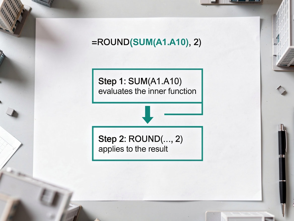
Yes. ROUND nests cleanly inside any Excel formula that accepts a number as an argument. Common patterns include =ROUND(SUM(A1:A100), 2) to round a sum, =ROUND(A1*B1, 2) to round a product, and =ROUND(IF(A1>0, A1*0.1, 0), 2) to round a conditional result. Excel supports up to 64 levels of function nesting, so you can embed ROUND as deeply as your formula logic requires. Nesting ROUND around a final calculation rather than at each intermediate step is the recommended approach for maintaining precision throughout the formula chain.

Nesting ROUND around a SUM is cleaner than rounding each input individually and preserves full intermediate precision.
Conclusion
The difference between =ROUND(A1,2) and simply formatting a cell to display 2 decimal places is not cosmetic: it determines whether your financial model’s totals reconcile to the cent or silently accumulate rounding discrepancies. Use ROUND (and its directional variants ROUNDUP, ROUNDDOWN, MROUND) when the stored value must be precise. Use Format Cells when you need clean visual presentation without altering the underlying data. Apply rounding at the final output stage, not mid-chain, to keep intermediate calculations at full precision.
For professional-grade financial models that follow these rounding conventions consistently across income statements, cash flow projections, and valuation outputs built to GAAP and IFRS presentation standards, consider downloading templates that embed these best practices throughout.