
0 ITEMS

Data Centre Project Finance & Colocation Model – Power-Constrained Capacity, DSCR Debt Sizing (Excel)
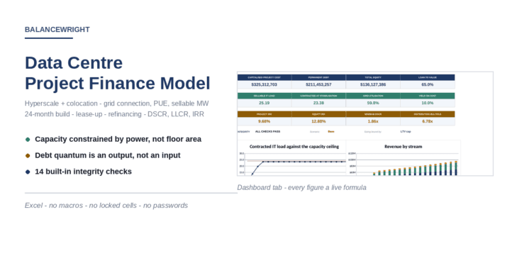
Data centre project finance model where the grid connection and design PUE set the sellable IT load: a contracted-load book built through lease-up and churn, a permanent facility sized on DSCR capacity and an LTV cap, twenty years of cash flow, an exit on a cap rate, and fourteen integrity checks. Twelve tabs, live formulas, no macros and no circular references.
| Financial Model, Infrastructure, Real Estate |
| Debt Schedule, Debt Service Coverage, Excel, IRR (Internal Rate of Return), NPV (Net Present Value), Project Finance |
Almost every data centre model in circulation is a real estate model with the words “data centre” on the cover. It takes square feet, applies a rent, escalates it, subtracts an operating cost ratio and capitalises the result. That works for an office block. It does not work here, because this asset is not constrained by floor area. It is constrained by the megawatts the utility has agreed to deliver.
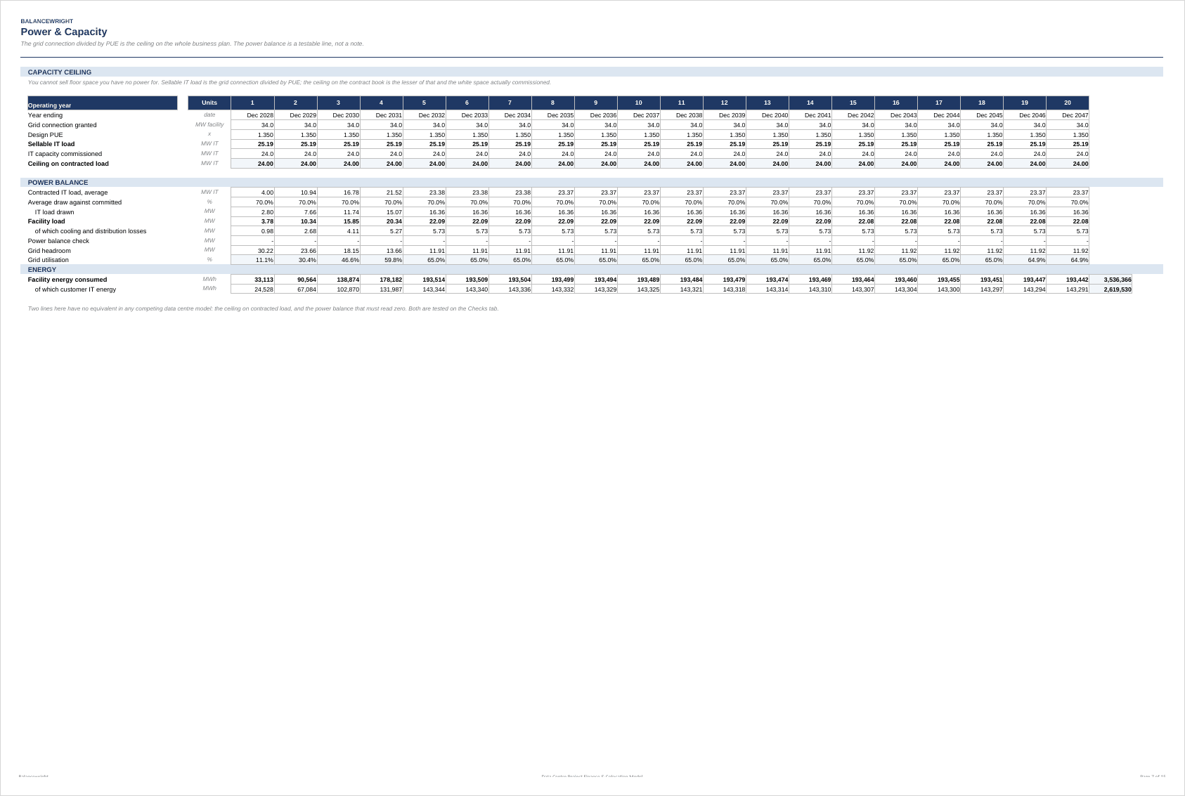
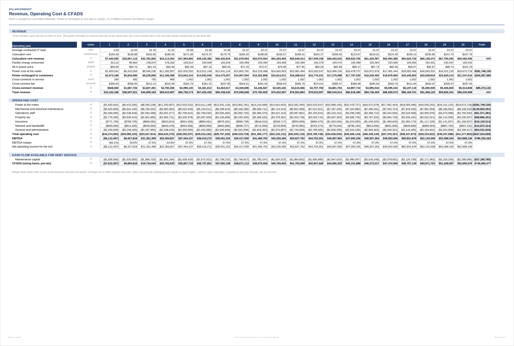
Power is the binding constraint. The grid connection divided by design PUE gives the IT load you can actually sell – cooling, distribution and losses take the difference – and that figure is a hard ceiling no lease-up plan can breach. Contracted IT load times the average customer draw gives the load drawn; that times PUE gives facility load; facility load against the connection gives headroom. The Checks tab tests, on every one of the twenty operating years, that the headroom is not negative and that the power balance reconciles exactly. Revenue then follows from the same quantities rather than from an unrelated rent roll: rent on committed IT load, metered energy recharged at cost plus a margin, and cross-connects per megawatt contracted.
No circular references. Twenty-four monthly construction columns take the capital spend through an S-curve you control, fund it at your target gearing, and capitalise the arrangement fee, the commitment fee and the interest during construction month by month. Because interest is charged on the balance at the start of each month, the ledger resolves left to right – no cell depends on itself, and iterative calculation stays switched off.
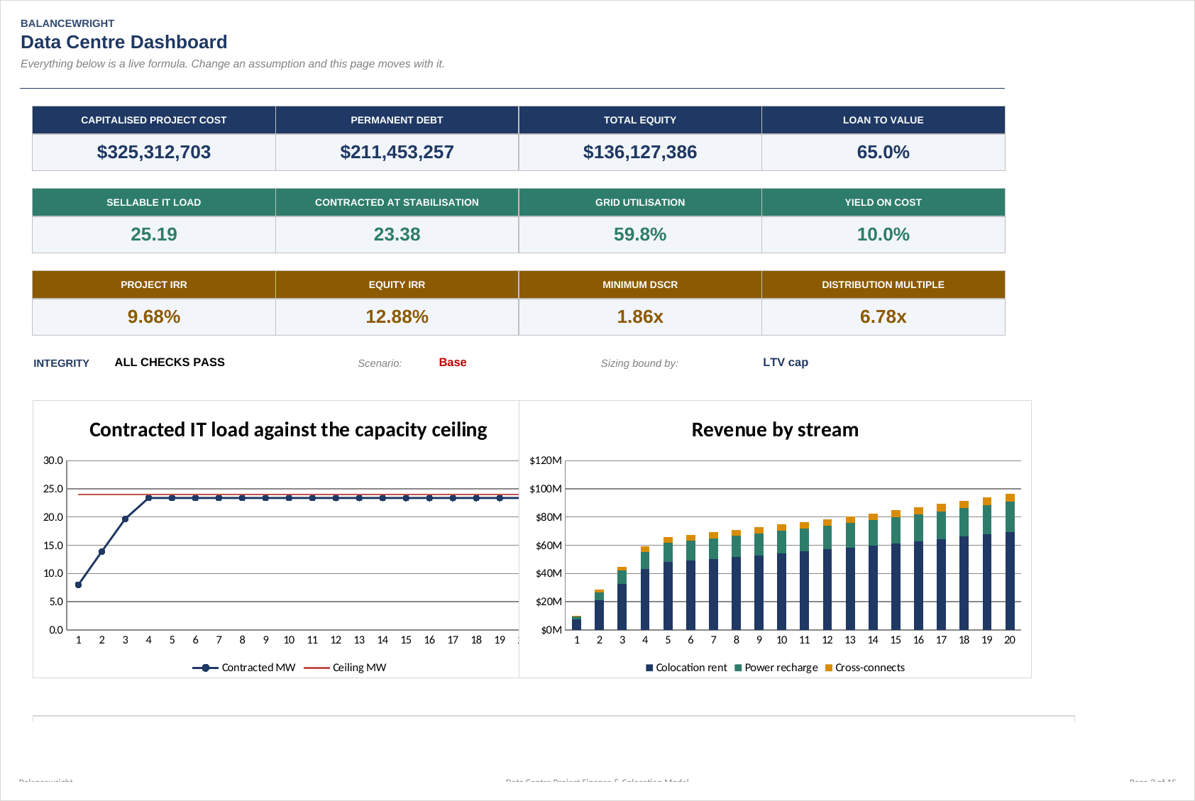
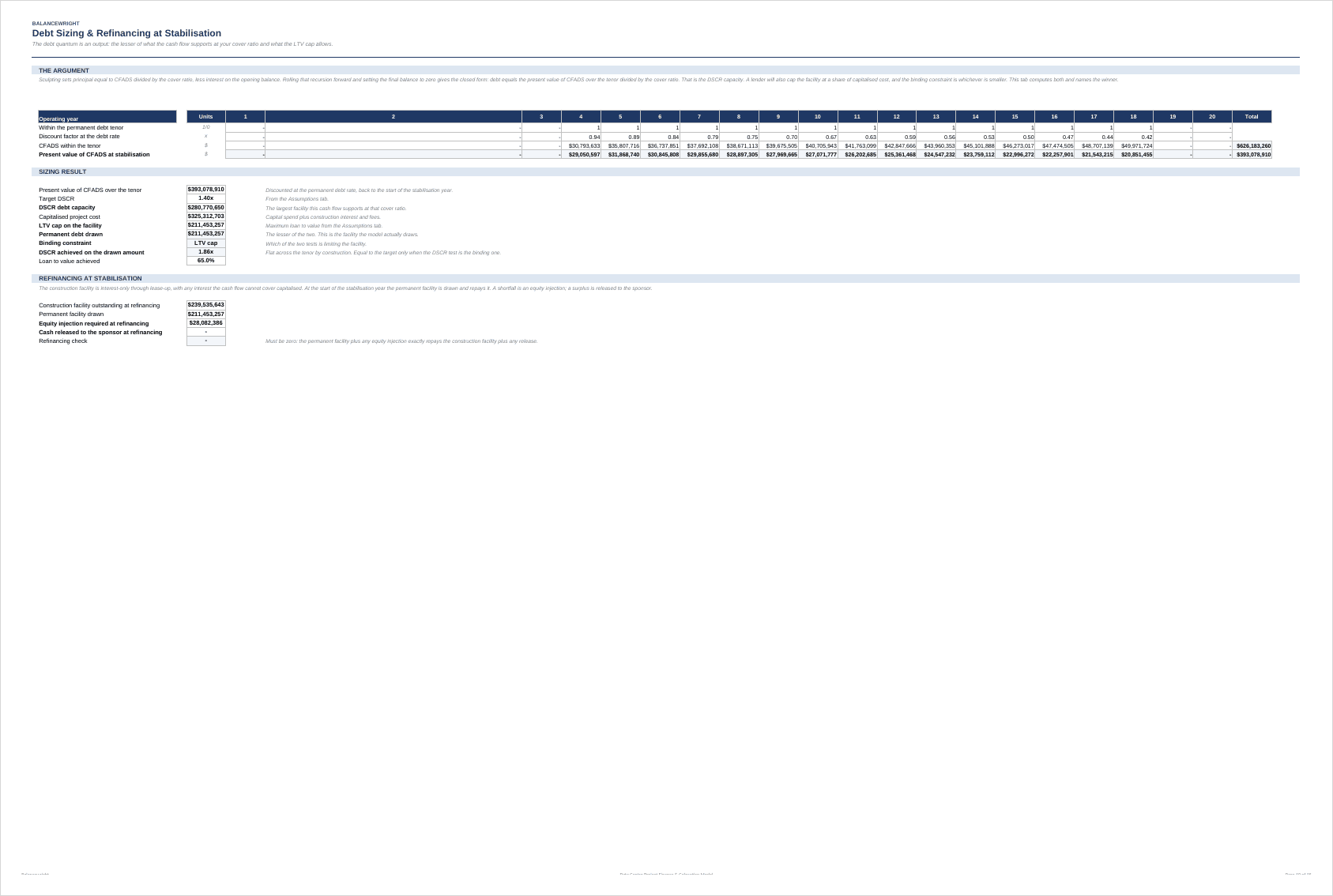
Debt is an output, not an input. A lender runs two tests and lends the lesser of them: what the cash flow services at a target cover ratio, and what the asset supports as a share of cost. The model computes the DSCR capacity in closed form – the present value of CFADS over the tenor divided by the target ratio, one division, no goal seek and no solver – computes the loan-to-value cap on capitalised project cost, draws the lesser of the two, and names the binding constraint in words on the Dashboard.
Lease-up and the refinancing in between. The construction facility remains outstanding on an interest-only basis while the hall fills, with any interest the ramping cash flow cannot pay capitalised rather than assumed away. At the start of the stabilisation year the permanent facility is sized on the stabilised cash flow and drawn to repay it: a shortfall is an equity injection the model shows you, a surplus is released to the sponsor, and the Checks tab reconciles the refinancing to the cent.
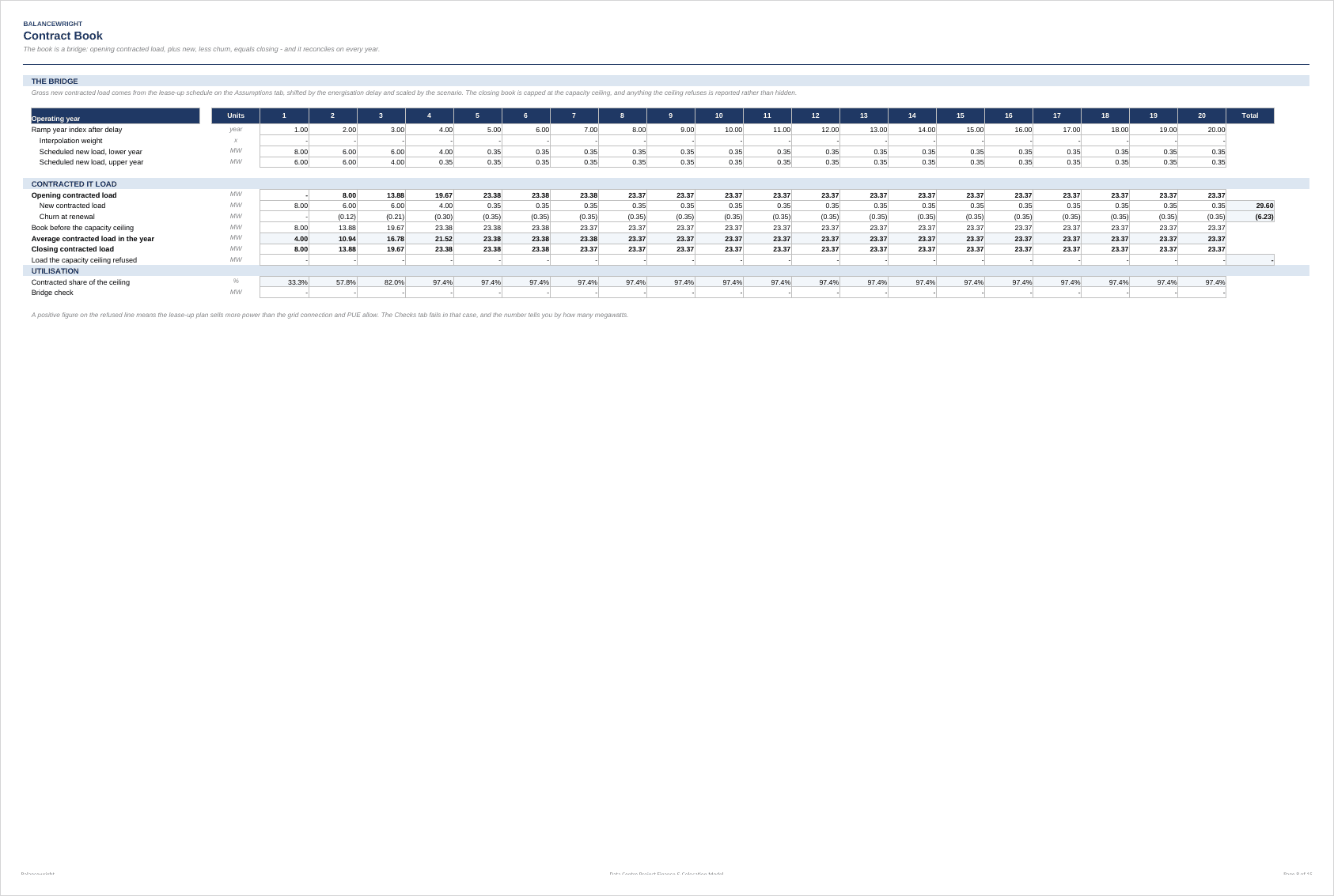
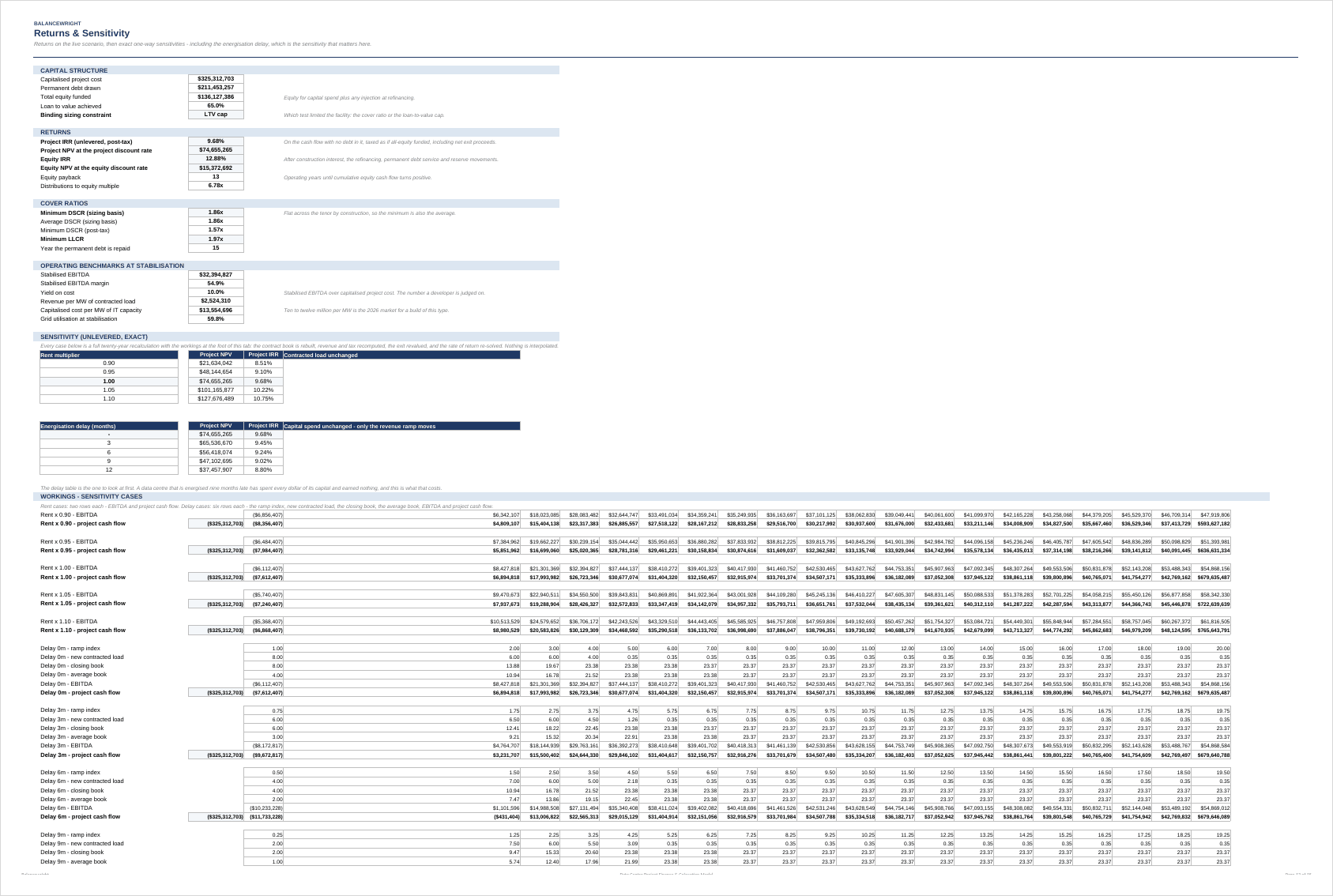
The contract book is a bridge, not a typed-in row. Opening contracted load plus new contracts less churn equals the closing book, capped by the power ceiling, with the average book carrying revenue and the whole ramp shifted by an energisation delay you can set. That delay is the sensitivity that matters on a data centre in this market, and it is one of two exact one-way tables on the Returns tab: every case rebuilds the contract book, recomputes revenue, cost and tax, revalues the exit and re-solves the rate of return, with the workings on the same tab so you can audit them.
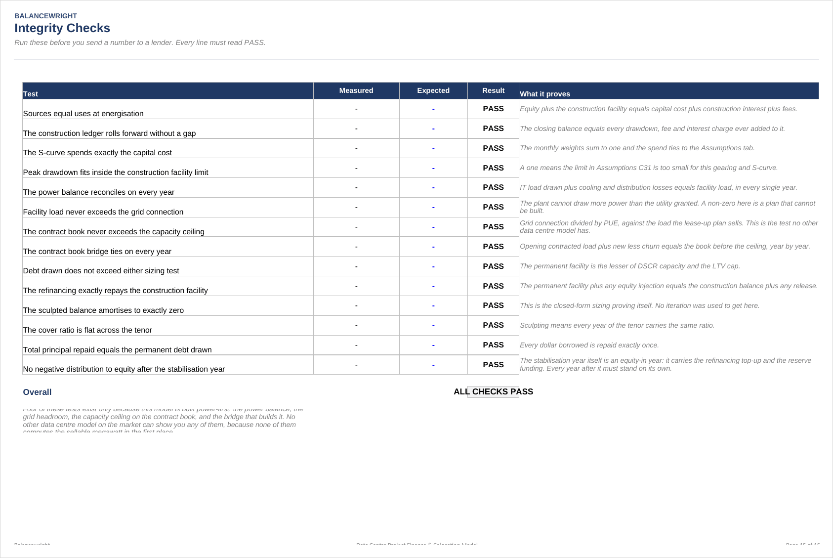
Fourteen integrity checks have to read PASS before any of it is worth quoting. Four of them exist only because this model treats the asset as a power business: the power balance reconciles every year, facility load never exceeds the grid connection, the contract book never exceeds the capacity ceiling, and the book bridge ties year by year. A model built on floor area cannot run them, because it never computes the quantities they test.
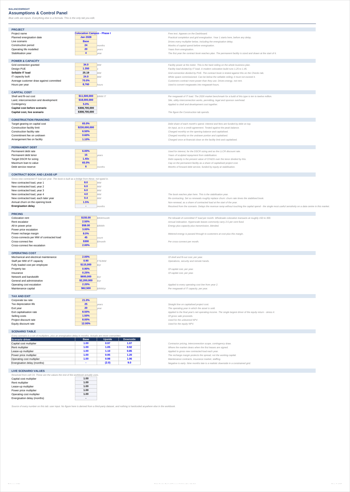
What is inside. Twelve tabs: Read Me, Dashboard, Assumptions, Construction & Funding, Power & Capacity, Contracted Capacity, Revenue & Costs, Debt Sizing, Debt Schedule, Cash Flow, Returns, Checks. Live formulas throughout. No macros, no add-ins, no external links, no locked cells and no passwords. A worked example is pre-loaded – a 34 MW connection at 1.35 PUE, 24 MW of IT capacity built, leased up over four years at $155 per kW per month – so every tab works the moment you open it. A nine-page PDF guide covers the method, the three inputs people get wrong, and the limitations stated plainly.
Outputs. Project and equity IRR and NPV, equity payback and distribution multiple, minimum and average DSCR, minimum LLCR, yield on cost, grid utilisation, revenue per megawatt and EBITDA margin – with a Base, Upside and Downside scenario switch that re-sizes the debt as well as the revenue.
Similar ProductsOther customers were also interested in...



 eFinancialModels
Electric Vehicle (EV) Charging Station Financial M...
With this comprehensive 5- or 10-year monthly tool, investors can assess the viability of setting up... Read more

Financial Model for Mobile App | Mobile App Busine...
The Mobile App Financial Plan Template in Excel allows you to develop financial projections when lau... Read more

 HenrySheykin
Food Truck Financial Model Excel Template
The Food Truck Financial Model helps entrepreneurs, founders, business owners, consultants, and anal... Read more

Green Hydrogen Production from Wind Energy Financi...
The Green Hydrogen from Wind Financial Model aims to comprehensively forecast a horizon of 40 years ... Read more

Simple Mutual Non-Disclosure Agreement Template
Protect your business secrets with ease using our Simple Mutual Non-Disclosure Agreement Template. S... Read more

Solar Energy Financial Model
The Solar Energy Financial Model Spreadsheet Template in Excel assists you in preparing a sophistica... Read more

 Peter Graf
The Customer-Centric Financial Model for Restauran...
Starting a restaurant without a financial plan is like driving a car blindfolded. You wouldn´t do i... Read more
You must log in to submit a review.