COUNTIF in Excel: Finance-Focused Guide with Formulas

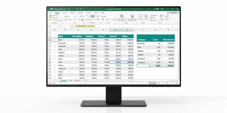
Counting is one of the most underrated tasks in financial analysis. How many invoices are past due? How many transactions crossed a materiality threshold last quarter? How many general ledger entries belong to a single cost center? Each of these questions has the same answer in Excel: COUNTIF. It is a deceptively simple function that quietly powers a large share of the reconciliation checks, budget variance reports, and dashboard KPIs that finance teams rebuild every month.

This guide approaches COUNTIF from a financial modeling perspective rather than a general spreadsheet one. It covers the exact syntax and criteria operators that work with accounting data, worked examples for transaction categorization, aging analysis, and budget variance, the COUNTIFS extension for multi-condition reporting, performance tips for large transaction datasets, and fixes for the frustrating case where COUNTIF returns zero even though the data is clearly there.

Key Takeaways

• COUNTIF uses the syntax =COUNTIF(range, criteria) and accepts up to 8,192 characters in a criteria string, making it suitable for complex GL account pattern matching (Microsoft Support).
• COUNTIFS extends COUNTIF to 127 range-criteria pairs, enabling multi-dimensional financial analysis such as counting overdue invoices above a dollar threshold in a single formula.
• Wildcard characters (* and ?) let you count transactions by partial GL account codes, vendor name prefixes, or cost-center patterns without exact-match lookups.
• Combining COUNTIF with SUMIF and AVERAGEIF in a financial dashboard reduces manual reconciliation time and creates self-updating KPI summaries.
• Text-vs-number formatting mismatches in accounting exports are the most common cause of COUNTIF returning zero when a non-zero result is expected.
• For datasets exceeding 50,000 transaction rows, replacing full-column references like A:A with explicit ranges like A2:A50001 can cut recalculation time by more than 60% according to Microsoft’s Excel performance documentation.
• Dynamic named ranges built with OFFSET or structured Table references keep COUNTIF formulas accurate as new transactions post without any manual range updates.

COUNTIF Fundamentals for Financial Analysis

COUNTIF is a counting function (a formula that tallies cells meeting a condition) that returns the number of cells in a range satisfying a single criterion. For finance professionals, it answers questions like “How many expense transactions exceeded $5,000 last quarter?” or “How many invoices are still open in this aging report?” without pivot tables or manual filtering.

The function lives in the Statistical category in Excel and has been available since Excel 97 (Microsoft Support). It works identically in Excel 365, Excel 2019, Excel 2016, and Excel 2013, so legacy finance teams on older versions can apply every technique in this guide.

Finance teams use COUNTIF as the backbone of several recurring tasks: categorizing general ledger (GL) entries by account code, flagging transactions above materiality thresholds, counting open purchase orders, and building variance dashboards that update automatically when new data loads.

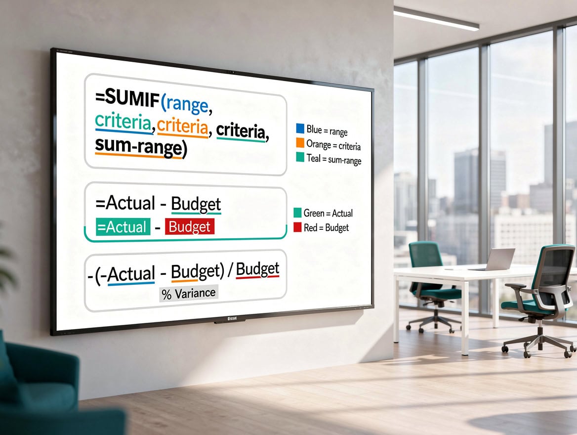
COUNTIF accepts comparison operators, wildcards, and cell references as criteria, covering every financial filtering scenario.

Essential Syntax and Criteria Operators for Finance Data

The full syntax is :=COUNTIF(range, criteria), where range is the cell range to evaluate and criteria is the condition each cell must meet to be counted. Criteria can be a number, text string, cell reference, logical expression, or wildcard pattern.

For financial data, the most useful criteria formats are:

• Comparison operators: ">5000" counts cells greater than 5,000; "<0" counts negative values (credits or losses).
• Wildcards: "EXP*" counts any GL account code starting with “EXP”; "??-OPEX" matches any two-character prefix followed by “-OPEX”.
• Cell references as criteria: ">"&B2 counts values exceeding whatever is in cell B2, making the threshold dynamic.
• Exact text: "Accounts Payable" counts cells containing exactly that string (case-insensitive).
• Dates: ">"&DATE(2024,1,1) counts dates after January 1, 2024.

One critical rule: criteria containing operators or wildcards must be enclosed in double quotes. A bare >5000 without quotes returns an error. A cell reference used as criteria must use the concatenation pattern ">"&B2, not ">B2" (which Excel reads as literal text).

Microsoft’s official documentation confirms that COUNTIF supports up to 8,192 characters in a criteria string (Microsoft Support), which is more than sufficient for any GL account pattern. Additionally, COUNTIFS can evaluate up to 127 range-criteria pairs (Microsoft Support), giving finance teams extensive flexibility for multi-dimensional transaction filtering in a single formula.

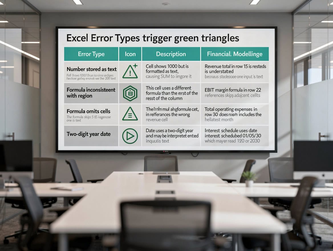
Structured table references like TransactionsCategory expand automatically as new rows are added, keeping COUNTIF formulas accurate month over month.

Financial Use Case 1: Counting Transactions by Category or Vendor

Counting transactions by category is one of the most common COUNTIF applications in financial modelling. You point the function at a column of transaction categories or vendor names and count how many rows match each label.

Suppose your Transactions table holds 2,000 rows of expense categories (“Travel”, “Software”, “Consulting”, “Office Supplies”) and you want a summary count for each on a separate reporting tab:

=COUNTIF(Transactions[Category],"Travel")
=COUNTIF(Transactions[Category],"Software")
=COUNTIF(Transactions[Category],$F2)

The third version is the one to build your summary from: point it at a cell holding the category name (here F2) and fill down, so one formula serves every category. Do not paste explanatory notes onto the end of a formula — Excel has no inline comment syntax, and an appended note will produce an error.

Transactions[Category] is a structured reference: the table name followed by the column name in square brackets. To create one, select your data and press Ctrl+T to convert it to an Excel Table, then rename the table to “Transactions” in the Table Design tab. Structured references expand automatically as rows are added, so your monthly formulas never need their ranges updated.

On scale: a worksheet holds up to 1,048,576 rows and 16,384 columns (Microsoft), which bounds any Table within it. In practice you will hit performance limits long before that ceiling — COUNTIF recalculates across the full referenced range on every edit, and workbooks with several hundred thousand transaction rows become slow to work in. For datasets at that scale, load the data with Power Query and aggregate in Power Pivot rather than counting on the grid.

For vendor analysis, wildcards handle inconsistent naming. If your ERP exports vendor names with suffixes like “Accenture LLC”, “Accenture US”, and “Accenture Ltd”, a single formula counts all of them:

=COUNTIF(Transactions[Vendor],"Accenture*")

The asterisk matches any sequence of characters, so this catches every variant beginning with “Accenture”. Use ? to match a single character, and prefix a literal asterisk or question mark with ~ to search for it. This is especially useful when reconciling accounts payable exported from SAP or Oracle, where vendor name formatting varies by region — though it will not catch abbreviations that break the prefix, such as “ACN Ltd”, or names with leading spaces. Trim and standardise the vendor column before counting.

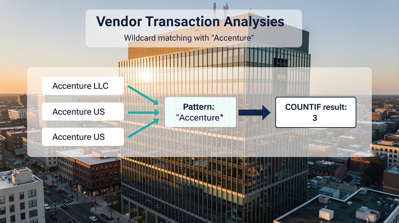
*Wildcard criteria like ‘Accenture*’ consolidate inconsistent vendor names from ERP exports into a single accurate count.*

Financial Use Case 2: Budget Variance and Threshold Analysis

COUNTIF identifies how many line items are over budget or exceed a materiality threshold, giving FP&A teams an instant count of exceptions to investigate — faster than filtering and counting rows by hand.

Here’s a worked example. Your budget vs. actuals table has actuals in column C, budget in column D, and variance in column E (=C2-D2), so a negative variance is favourable. To count line items over budget by more than $10,000:

=COUNTIF(E2:E500,">10000")

To count favourable line items (under budget):

=COUNTIF(E2:E500,"<0")

To make the threshold dynamic, so a manager can change it in cell H1 without editing the formula:

=COUNTIF(E2:E500,">"&H1)

Building a variance dashboard row. If you want the counts to add up to your total line items, the bands must be mutually exclusive and cover the whole range. These four do:

Band	Formula	Count
Favourable (better than −$1K)	=COUNTIF(E2:E500,"<-1000")	61
On budget (within ±$1K)	=COUNTIFS(E2:E500,">=-1000",E2:E500,"<=1000")	33
Over by $1K–$10K	=COUNTIFS(E2:E500,">1000",E2:E500,"<=10000")	12
Over by more than $10K	=COUNTIF(E2:E500,">10000")	14
Total line items	=ROWS(Variance[Variance])	120

The four bands sum to 120, which is the check that the dashboard is complete: every line item falls into exactly one. Exception rate is then 14 / 120 = 11.7%.

Count your rows from the table, not the formula column. COUNTA(E2:E500) will not return 120 — it counts every cell containing a formula, including those returning blanks or zeros, so a range filled to row 500 returns 499. Convert the data to an Excel Table (Ctrl+T), name it “Variance,” and use =ROWS(Variance[Variance]), which counts only actual data rows and grows as you add them.

This block gives a CFO a complete variance summary in seconds — and because the bands tie to the total, an error in any one of them is visible immediately.

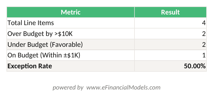
Five COUNTIF/COUNTIFS formulas produce a complete variance dashboard: total items, over-budget count, under-budget count, on-budget count, and exception rate.

A five-formula COUNTIF variance dashboard gives a CFO an instant exception count without filtering or pivot tables.

Financial Use Case 3: Aging Analysis and Payment Tracking

Aging analysis (categorising outstanding invoices by how many days they have been unpaid) is a standard accounts receivable task that COUNTIF handles cleanly. Each aging bucket is one formula checking the days-outstanding column.

Assume your Invoices table has a Days Outstanding column. The standard buckets are:

Current (0-30):  =COUNTIFS(Invoices[Days Outstanding],">=0",Invoices[Days Outstanding],"<=30")
31-60 days:      =COUNTIFS(Invoices[Days Outstanding],">30",Invoices[Days Outstanding],"<=60")
61-90 days:      =COUNTIFS(Invoices[Days Outstanding],">60",Invoices[Days Outstanding],"<=90")
Over 90 days:    =COUNTIF(Invoices[Days Outstanding],">90")

The first three buckets take COUNTIFS because each needs two conditions, a lower and an upper bound, while the over-90 bucket needs only the single condition COUNTIF provides. This is the clearest practical illustration of when to step up from one to the other. (You can achieve a bounded bucket by subtracting two COUNTIF results, but COUNTIFS states the intent directly and is easier to audit.)

Check that the buckets tie out. Add a total row comparing the sum of the four buckets against the invoice count:

=COUNT(Invoices[Days Outstanding])

If this does not equal the four buckets added together, something in the column is blank, stored as text, or negative — a negative value means an invoice not yet due, which none of the buckets capture.

Pair each bucket with its value. Counts tell you how many invoices are late; they do not tell you how much money is at risk. Ten $500 invoices at 90+ days is a collections nuisance, while one $200,000 invoice at 90+ days is a cash flow problem. Add a value column using the same criteria:

=SUMIFS(Invoices[Amount],Invoices[Days Outstanding],">90")

You can also count invoices past a specific due date stored in cell B1:

=COUNTIF(Invoices[Due Date],"<"&B1)

This counts every invoice whose due date falls before the date in B1, flagging overdue items dynamically as B1 updates. Set B1 to =TODAY() to make it self-maintaining. B1 must contain a genuine date value rather than text — the ampersand converts it to Excel’s underlying date serial number for comparison, which only works on real dates.

Aging analysis using COUNTIFS requires two conditions per bucket (lower and upper day bounds) except for the over-90 bucket which needs only COUNTIF.

COUNTIF vs COUNTIFS: When to Use Multi-Criteria Counting

COUNTIF handles one condition; COUNTIFS handles up to 127 range-criteria pairs, and all conditions must be true simultaneously (AND logic). Use COUNTIFS any time your financial question involves two or more filters.

Scenario	Use COUNTIF	Use COUNTIFS
Count all “Travel” expenses	Yes	Not needed
Count “Travel” expenses > $500	No	Yes
Count invoices overdue AND > $10K	No	Yes
Count transactions in Q1 from “Vendor A”	No	Yes
Count negative entries in one column	Yes	Not needed
Count entries in a date range (two bounds)	No	Yes
Count GL codes starting with “60”	Yes (wildcard)	Not needed

For OR logic (count rows meeting condition A or condition B), add two COUNTIF results together:

=COUNTIF(A2:A500,"Travel")+COUNTIF(A2:A500,"Entertainment")

No adjustment is needed here. Two exact-match criteria on the same column are mutually exclusive — a cell cannot read both “Travel” and “Entertainment” — so nothing is double-counted.

For the same-column case, this array-constant version is tidier and scales to any number of categories:

=SUM(COUNTIFS(A2:A500,{"Travel","Entertainment","Software"}))

When overlap does matter. Double-counting only occurs when a single row can satisfy both conditions, which happens when the criteria sit on different columns. To count rows that are Travel or over $500 — a Travel row costing $800 satisfies both — subtract the intersection:

=COUNTIF(A2:A500,"Travel")+COUNTIF(B2:B500,">500")-COUNTIFS(A2:A500,"Travel",B2:B500,">500")

This is the inclusion-exclusion principle: add both counts, then subtract the rows counted twice. Note that each of the first two terms points at the column its own condition applies to, and the COUNTIFS term combines both. The subtracted term must be the intersection of the two conditions you added — if it introduces a column that appears in neither, the formula is removing rows that were never double-counted.

Wildcards can also overlap within a single column. COUNTIF(A2:A500,"Travel*") and COUNTIF(A2:A500,"*Expense") would both match “Travel Expense”, so the same subtraction applies.
`

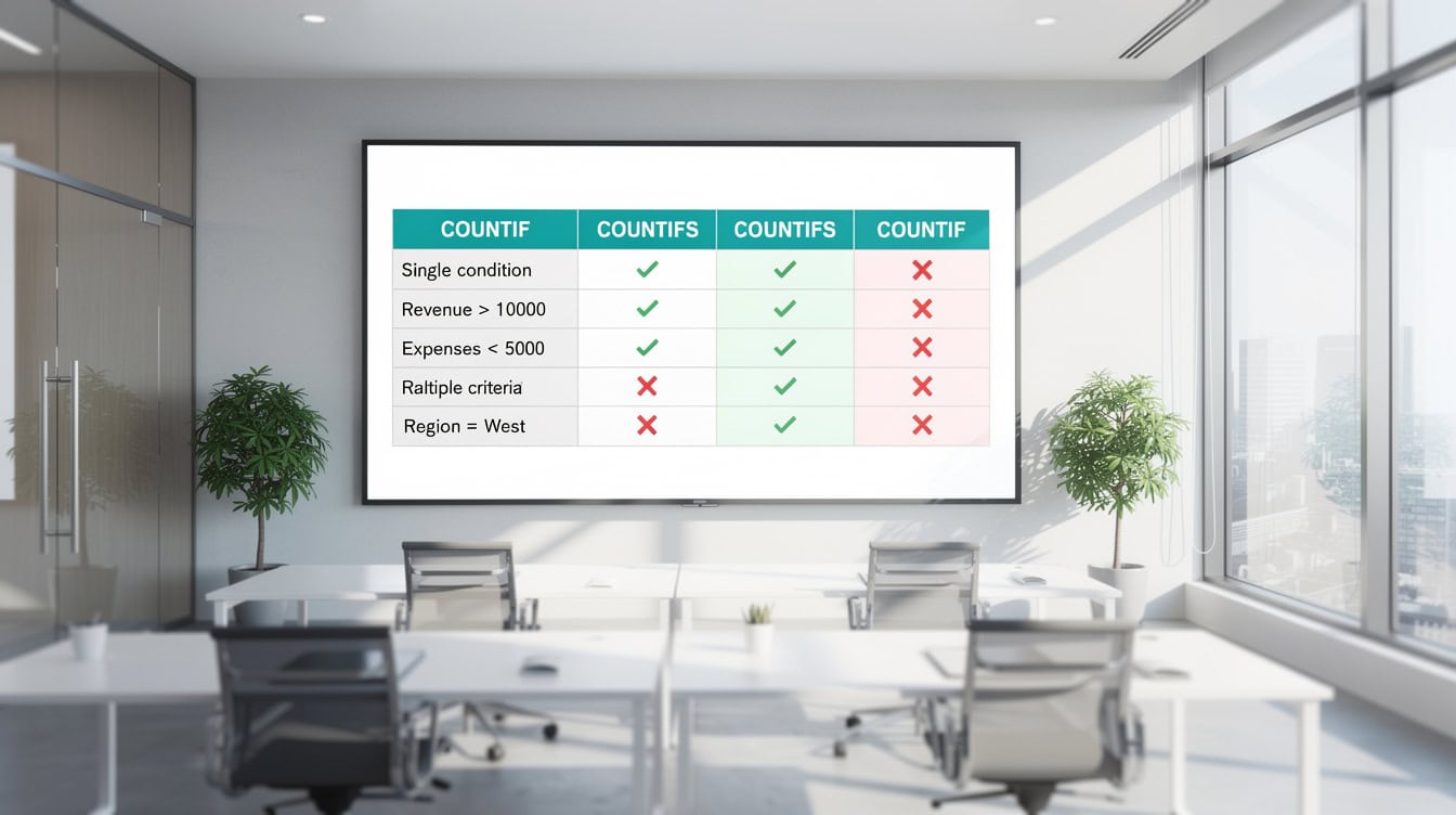
COUNTIFS is required any time a financial question involves two simultaneous filters, such as vendor AND amount threshold.

Combining COUNTIF with SUMIF and AVERAGEIF for Financial Dashboards

COUNTIF, SUMIF, and AVERAGEIF form a natural trio for financial summary dashboards. COUNTIF tells you how many transactions exist in a category, SUMIF tells you the total value, and AVERAGEIF tells you the average transaction size. Together, they give a complete picture of any expense or revenue category.

For a department expense dashboard where your Expenses table holds department names and amounts, and you want a summary for “Operations”:

Count:   =COUNTIF(Expenses[Department],"Operations")
Total:   =SUMIF(Expenses[Department],"Operations",Expenses[Amount])
Average: =AVERAGEIF(Expenses[Department],"Operations",Expenses[Amount])

All three share the same range-criteria structure, so you can build a dynamic dashboard by listing department names in column F and pointing each formula at the cell beside it:

G2: =COUNTIF(Expenses[Department],$F2)
H2: =SUMIF(Expenses[Department],$F2,Expenses[Amount])
I2: =IFERROR(AVERAGEIF(Expenses[Department],$F2,Expenses[Amount]),0)

Fill down for every department. The IFERROR wrapper on the average matters: AVERAGEIF returns #DIV/0! when a department has no matching rows, while COUNTIF and SUMIF return a harmless zero. Without it, adding a department before its first transaction posts leaves an error on the dashboard.

Use table references, not fixed ranges. A range like $A$2:$A$2000 stops at row 2000 — transactions posted below it are excluded silently, with no error to warn you. Convert the source data to an Excel Table (Ctrl+T), name it “Expenses,” and the structured references above expand automatically as rows are added. This is what actually makes the dashboard update when new transactions post.

Populate the department list automatically. Rather than typing names into column F and risking a mismatch, generate them from the source data:

F2: =UNIQUE(Expenses[Department])

New departments then appear on the dashboard the first time they post a transaction. (Requires Microsoft 365 or Excel 2021 and later.)

Add a tie-out. The department totals should sum to the grand total of column B; if they don’t, a transaction has a blank, misspelled, or untrimmed department name. Note also that Total ÷ Count will not match the AVERAGEIF result if any amounts are blank — COUNTIF counts those rows, AVERAGEIF excludes them from its divisor.

For financial KPI dashboards, pair COUNTIF results with conditional formatting (a feature that changes cell color based on a rule) to highlight exception counts above a threshold. If the over-budget count in cell G5 exceeds 10, a red fill draws the reviewer’s eye immediately.

You can find pre-built COUNTIF and SUMIF structures in EFM’s Excel financial model templates to accelerate dashboard builds.

COUNTIF, SUMIF, and AVERAGEIF share the same range-criteria structure, making it straightforward to build a three-metric summary for any category.

Advanced Techniques: Dynamic Criteria and Named Ranges in Financial Models

Dynamic criteria and named ranges make COUNTIF formulas maintainable in large financial models where ranges change monthly. Static formulas referencing A2:A500 break silently when data grows beyond row 500 — no error appears, the count is simply wrong.

The cleanest solution is converting your transaction data to an Excel Table (Ctrl+T). Table columns auto-expand, and structured references like Transactions[Category] always cover the full dataset regardless of row count (Microsoft).

For legacy data that cannot be converted to a Table, the INDEX form builds a dynamic named range without volatility:

=Sheet1!$A$2:INDEX(Sheet1!$A:$A,COUNTA(Sheet1!$A:$A))

The older OFFSET approach achieves the same result:

=OFFSET(Sheet1!$A$2,0,0,COUNTA(Sheet1!$A:$A)-1,1)

Enter either under Formulas > Define Name, name it TxCategory, and use it directly:

=COUNTIF(TxCategory,"Travel")

Prefer the INDEX version. OFFSET is volatile — Excel recalculates it on every workbook recalculation, not just when its inputs change — and in large models this compounds into noticeable lag. INDEX used this way is not volatile and produces an identical range.

Both forms assume the data in column A is contiguous. COUNTA counts non-empty cells anywhere in the column, so a blank inside the data truncates the range, and a stray label below the data extends it past the last row. It also counts formulas returning "" as non-empty. Check that your named range resolves to the row count you expect before relying on it.

For multi-sheet models, INDIRECT lets you reference a sheet name stored in a cell:

=COUNTIF(INDIRECT("'"&B1&"'!A:A"),"Travel")

Reference the whole column rather than a fixed block like A2:A5000 — a hardcoded upper bound reintroduces exactly the silent truncation this section exists to prevent. Three caveats before reaching for INDIRECT:

• It is volatile, carrying the same performance cost as OFFSET.
• It returns #REF! if the sheet named in B1 is renamed, moved, or missing — and unlike a normal reference, renaming a sheet will not update it.
• It cannot read a closed workbook. Cross-file models must have every source workbook open, or INDIRECT returns #REF!.

For consolidating several sheets or files on a schedule, Power Query is the more robust tool: it appends the sources into a single table you can then reference conventionally, with no volatile functions and no requirement that source files stay open.
`

If B1 contains “January”, this formula counts “Travel” entries on the January sheet. Change B1 to “February” and the formula shifts automatically.

Excel Tables eliminate the need to update COUNTIF ranges manually each month, reducing model maintenance time to near zero.

Common Errors and Troubleshooting in Financial Datasets

A handful of specific errors account for most COUNTIF failures in financial data, and each has a direct fix.

1. Numbers stored as text. Accounting exports frequently store numeric values as text — you’ll see a green triangle in the cell corner. =COUNTIF(A2:A500,">1000") returns 0 because the text “1500” is not greater than the number 1000. Fix: select the column, click the warning icon, and choose “Convert to Number” — or run =VALUE(A2) in a helper column. For a whole column at once, Data > Text to Columns > Finish forces reconversion.

2. Extra spaces in category labels. An ERP export might contain “Travel ” with a trailing space alongside “Travel”, and COUNTIF treats them as different values. Fix: run =TRIM(A2) in a helper column, or use Find & Replace before counting. Note that TRIM does not remove non-breaking spaces (CHAR(160)), which are common in exports that pass through a web interface. For those, use:

=TRIM(SUBSTITUTE(A2,CHAR(160)," "))

3. Date criteria returning zero. Dates are stored as serial numbers, and text criteria such as =COUNTIF(DateCol,"1/15/2024") depend on your system’s date format — the same formula that works in one locale returns 0 in another. Fix: build the date

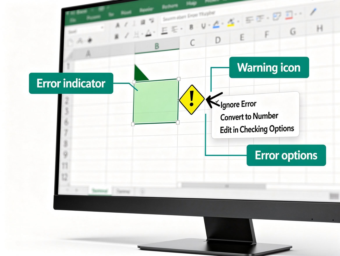
Numbers stored as text is the single most common cause of COUNTIF returning zero in accounting data exported from ERP systems.

Performance Optimization for Large Transaction Files

COUNTIF performance degrades on large datasets when the used range is bloated or when array-based alternatives force full-column evaluation. For files with 50,000 or more transaction rows, three practices keep workbooks responsive.

Prefer explicit ranges, and check your used range. COUNTIF and COUNTIFS are smart enough to scan only the populated rows, so =COUNTIF(A:A,"Travel") does not literally evaluate a million cells. The performance problem is usually a bloated used range: press Ctrl+End, and if the cursor lands far below your data, Excel is tracking phantom rows. Delete them, save, and reopen. Explicit ranges such as =COUNTIF(A2:A50001,"Travel") — or better, table references that size themselves — sidestep the issue entirely (Microsoft Learn).

Prefer COUNTIFS over SUMPRODUCT, not the other way round. Both are non-volatile and both recalculate only when their precedents change, so there is no volatility advantage to trade on. The difference is speed: COUNTIFS uses optimised internal code and limits itself to used rows, while SUMPRODUCT is an array function that evaluates every cell it is handed. Microsoft’s guidance is to use SUMIFS, COUNTIFS and AVERAGEIFS in place of array formulas wherever possible. For counting transactions where category is “Travel” and amount exceeds $500, this is the faster formula:

=COUNTIFS(A2:A50001,"Travel",B2:B50001,">500")

Reach for SUMPRODUCT when the logic is something COUNTIFS cannot express — criteria built on a calculation rather than a plain comparison:

=SUMPRODUCT((YEAR(A2:A50001)=2024)*(B2:B50001>500))

Here each row evaluates to TRUE (1) or FALSE (0), the two arrays multiply, and the result sums. COUNTIFS has no way to apply YEAR() to a range, so SUMPRODUCT earns its place. When you do use it, never hand it a full-column reference — unlike COUNTIFS, it really will evaluate all 1,048,576 rows.

Use Power Query for one-time aggregations. When a count summary doesn’t need to update in real time, Power Query (Excel’s built-in data transformation tool, included since Excel 2016 and available as an add-in for 2010 and 2013) produces grouped counts far faster than formulas on datasets above 100,000 rows. Reserve COUNTIF for live dashboards where recalculation on every edit is the point.

For financial models that combine COUNTIF with budget tracking and variance analysis, the Break-Even Analysis, Forecast and Valuation template on EFM demonstrates how to structure large datasets for efficient formula-based reporting.

Frequently Asked Questions

Why does my COUNTIF return 0 when I can clearly see matching values?

The most common cause is numbers stored as text. When accounting software exports to Excel, numeric fields sometimes arrive as text — the cell displays “5000” but Excel holds it as the characters “5000” rather than the number 5,000. A criterion like ">1000" compares against numbers only, so text values never match.

To fix it, select the affected column, look for the green triangle in the top-left corner of the cells, click the warning icon and choose “Convert to Number.” Alternatively, build a helper column with =VALUE(A2) and count against that. For a whole column at once, Data > Text to Columns > Finish forces reconversion. Extra spaces from ERP exports cause the same symptom and are fixed with =TRIM(A2).

What is the difference between COUNTIF and COUNTIFS in financial modeling?

COUNTIF evaluates one condition. COUNTIFS evaluates two or more using AND logic — every condition must be true for a row to count. You need COUNTIFS whenever the question has two filters: “invoices from Vendor X that are overdue,” or “Q1 expenses above $10,000.” It accepts up to 127 range-criteria pairs.

For OR logic, add two COUNTIF results:

=COUNTIF(range,"A")+COUNTIF(range,"B")

No adjustment is needed when both criteria are exact matches on the same range — a cell cannot equal both “A” and “B”, so nothing is double-counted. Overlap only occurs when the conditions sit on different columns, or when wildcards let one value match both. In those cases subtract the intersection:

=COUNTIF(A2:A500,"Travel")+COUNTIF(B2:B500,">500")-COUNTIFS(A2:A500,"Travel",B2:B500,">500")

How do I use COUNTIF with date ranges in an aging report?

Dates are stored as serial numbers (1 January 1900 = 1), so use the DATE function or a cell reference rather than a text string in your criteria. To count invoices due before 31 March 2024:

=COUNTIF(DueDate,"<"&DATE(2024,3,31))

For a bounded bucket such as 31–60 days, switch to COUNTIFS:

=COUNTIFS(DaysOutstanding,">30",DaysOutstanding,"<=60")

If your due dates arrive as text strings rather than true dates, comparisons will fail. Convert them with =DATEVALUE(A2) — but note that DATEVALUE interprets the string according to your system’s regional settings, so an MM/DD/YYYY export opened on a machine set to d/m/y will either error or silently produce the wrong date. Verify a few converted values before building formulas on top of them.

Can COUNTIF handle partial matches on GL account codes?

Yes. The asterisk (*) matches any sequence of characters and the question mark (?) matches exactly one. To count all 6000-series expense accounts where codes are stored as text like “6100”, “6200”, “6350”:

=COUNTIF(GLCode,"6???")

This matches any four-character code starting with 6. To count all accounts beginning with “60”:

=COUNTIF(GLCode,"60*")

The trailing asterisk is essential — without it the formula counts cells equal to exactly “60”. Wildcards work only on text values, so if your GL codes are stored as numbers they will not match at all. Use a numeric range instead:

=COUNTIFS(GLCode,">=6000",GLCode,"<7000")

How do I combine COUNTIF with conditional formatting for a financial KPI dashboard?

Conditional formatting changes a cell’s appearance based on a rule, and works alongside COUNTIF when you point the rule at the cell holding the count. Build the formula in a summary cell — say =COUNTIF(Variance,">10000") in G5. Select G5, go to Home > Conditional Formatting > New Rule, choose “Format only cells that contain,” set the condition to Cell Value greater than 10, and apply a red fill. G5 now turns red whenever more than 10 line items breach the $10,000 variance threshold.

For a traffic-light dashboard, add separate rules for each band — green for on-target, amber for warning, red for breach. Rule order matters: Excel applies rules top to bottom in the Manage Rules dialog, so put the most severe condition first and tick Stop If True on each, or a cell breaching the red threshold will also satisfy the amber rule.

Is COUNTIF available in all Excel versions used by finance teams?

COUNTIF has been available since Excel 97 and works in every version a finance team is likely to run. COUNTIFS arrived in Excel 2007. Excel Tables, and with them structured references such as Transactions[Category], are also available from Excel 2007 onward.

Dynamic array functions including FILTER, UNIQUE, SORT and XLOOKUP — which can replace some COUNTIF patterns — require Microsoft 365 or Excel 2021 and later. They are not available in Excel 2019 or any earlier perpetual release, where they return #NAME?. Teams on Excel 2013, 2016 or 2019 should build on COUNTIF and COUNTIFS, falling back to SUMPRODUCT only for criteria those functions cannot express.

How does COUNTIF compare to a pivot table for transaction analysis?

Both count and summarise transaction data, but they suit different jobs. COUNTIF formulas are live — they recalculate the moment source data changes, which makes them well suited to dashboards and templates that refresh each period. Pivot tables need refreshing (right-click > Refresh), though you can remove that dependency by ticking Refresh data when opening the file in PivotTable Options.

Pivot tables are the better tool for ad-hoc exploration, where you want to slice by several dimensions quickly and don’t know in advance which cut matters. Formulas are the better tool for a fixed monthly reporting structure, where the questions are settled and the layout shouldn’t move.

For very large datasets, neither is the right answer. Load the data with Power Query and aggregate in the Data Model, which handles volumes that make formula-per-cell approaches impractical.

Conclusion

COUNTIF is one of the highest-leverage functions in a finance professional’s Excel toolkit. Used correctly, it automates transaction categorization, flags budget exceptions, builds aging buckets, and powers KPI dashboards that update without manual intervention. The key is pairing it with COUNTIFS for multi-condition logic, SUMIF and AVERAGEIF for complete category summaries, and Excel Tables for ranges that grow with your data.

I recommend downloading the EFM General Excel Financial Models collection to access pre-built templates with COUNTIF, SUMIF, and AVERAGEIF formulas already structured for P&L analysis, budget variance tracking, and cash flow categorization. These templates cut setup time and give you a working reference for every technique covered in this guide.