0 ITEMS

Amortization Abbreviations: AMORT, AMZ + Excel Guide

Finance professionals use several abbreviations for amortization across financial models, accounting software, and regulatory filings, and choosing the wrong one can create confusion or conflict with other standard terms.
Key Takeaways
- The 3 accepted abbreviations for amortization in financial modeling are AMORT, AMZ, and AMTZ — never use AMT, which conflicts with Alternative Minimum Tax.
- Excel’s PMT function calculates the fixed monthly payment for a loan in a single formula: =PMT(rate/12, nper, -pv).
- A $250,000 mortgage at 6% APR over 30 years produces a monthly payment of $1,498.88 and total interest of $289,595.47.
- IRS Section 197 requires most acquired intangible assets to be amortized over a 15-year statutory period, regardless of actual useful life.
- FASB ASC 350 governs intangible asset amortization under US GAAP, distinguishing between finite-lived assets (amortized) and indefinite-lived assets (impairment-tested only).
- Amortization applies to intangible assets and loan balances; depreciation applies to tangible fixed assets — the distinction affects both the income statement and tax treatment.
- A 1-percentage-point increase in interest rate on a 30-year, $250,000 loan adds approximately $57,000 in total interest paid over the loan’s life.
Amortization Abbreviations in Financial Modeling: AMORT, AMZ, and Industry Standards
The standard abbreviations for amortization used in professional financial models and accounting software are AMORT, AMZ, and AMTZ. Each appears in different contexts, and using the correct one prevents misreading by auditors, lenders, and software systems.
AMORT is the most widely recognized shorthand. You’ll find it in Excel column headers, loan schedule tabs, and Big Four working papers. It’s unambiguous and readable at a glance.
AMZ appears frequently in financial modeling software and ERP systems where column width is constrained. Bloomberg terminal users and fixed-income analysts often use AMZ in bond amortization schedules.
AMTZ is a less common variant used in some accounting software exports and legacy systems. It’s functionally identical to AMORT but less intuitive for new readers.
Never use AMT as an abbreviation for amortization. AMT is the universally recognized abbreviation for Alternative Minimum Tax in US tax law, and using it for amortization creates serious ambiguity in any tax-adjacent financial model.
Under US GAAP, FASB ASC 350 governs the amortization of intangible assets with finite useful lives. Under IFRS, IAS 38 covers the same ground. Both standards require consistent application of the chosen amortization method across reporting periods, which means your abbreviation convention should also be consistent across all model tabs and financial statement footnotes.

AMORT, AMZ, and AMTZ are the three safe abbreviations; AMT is reserved for Alternative Minimum Tax under IRC Section 55.
Excel Amortization Formula Fundamentals: PMT, IPMT, and PPMT
Excel provides three dedicated functions for amortization schedule construction: PMT (total periodic payment), IPMT (interest portion of a payment), and PPMT (principal portion of a payment). Together, these three functions build a complete, self-reconciling amortization schedule. The PMT function accepts up to 5 arguments (Microsoft), making it flexible enough to handle standard loans, annuities due, and balloon structures within a single formula.
PMT syntax: =PMT(rate, nper, pv, [fv], type)
- rate: the periodic interest rate (annual rate divided by payment periods per year)
- nper: total number of payment periods
- pv: present value, or the loan principal (enter as a negative number to return a positive payment)
- fv: future value after the last payment (defaults to 0 for fully amortizing loans)
- type: 0 for end-of-period payments (standard), 1 for beginning-of-period
IPMT syntax: =IPMT(rate, per, nper, pv)
- per: the specific period number for which you want the interest component
PPMT syntax: =PPMT(rate, per, nper, pv)
- per: the specific period number for which you want the principal component
A critical check: for any period, IPMT + PPMT must equal PMT. If they don’t, you have a formula error. Microsoft’s function documentation confirms that IPMT and PPMT are mathematically complementary (Microsoft Support).
For variable-rate loans, replace the fixed rate argument with a cell reference that updates each period. This makes the schedule dynamic and allows sensitivity testing without rebuilding the table.

PMT, IPMT, and PPMT share the same core arguments; IPMT and PPMT add a ‘per’ argument to isolate a specific period’s interest or principal.
Building a Loan Amortization Schedule in Excel: Step-by-Step
A properly structured amortization schedule has six columns: Period, Beginning Balance, Payment, Interest, Principal, and Ending Balance. Build it in this exact order to ensure each row reconciles automatically.
Step 1: Set up the input block. In cells B1:B4, enter: Loan Amount ($250,000), Annual Rate (6%), Term in Years (30), and Payments per Year (12). This keeps all assumptions in one place for easy sensitivity testing.
Step 2: Calculate the fixed payment. In cell B6, enter: =PMT(B2/B4, B3*B4, -B1). This returns $1,498.88 for the base case.
Step 3: Build row 1 of the schedule. In the schedule table starting at row 10:
- Period (A10): 1
- Beginning Balance (B10): =$B$1 (links to the input block)
- Payment (C10): =$B$6 (fixed payment, locked reference)
- Interest (D10): =IPMT($B$2/$B$4, A10, $B$3$B$4, -$B$1)
- Principal (E10): =PPMT($B$2/$B$4, A10, $B$3$B$4, -$B$1)
- Ending Balance (F10): =B10-E10
Step 4: Build row 2 onward. In row 11:
- Beginning Balance (B11): =F10 (prior period ending balance)
- All other formulas copy down from row 10, with the period number in column A incrementing by 1.
Step 5: Validate. After copying down 360 rows (30 years × 12 months), the Ending Balance in the final row must equal zero (or within $0.01 due to rounding). Sum column C to verify total payments equal $539,595.47 for this example.

The six-column structure ensures each row self-reconciles: Beginning Balance minus Principal equals Ending Balance, which becomes the next row’s Beginning Balance.
Worked Example: $250,000 Mortgage at 6% Over 30 Years
Here’s the math for a $250,000 mortgage at 6% APR, monthly payments, 30-year term.
Monthly rate: 6% / 12 = 0.5% = 0.005
Number of periods: 30 × 12 = 360
Monthly payment formula:
M = P × r(1+r)^n / (1+r)^n – 1
M = 250,000 × 0.005 × (1.005)^360 / (1.005)^360 – 1
M = 250,000 × 0.005 × 6.02258 / 6.02258 – 1
M = 250,000 × 0.030113 / 5.02258
M = 250,000 × 0.005996
M = $1,498.88
First period breakdown:
- Interest: $250,000 × 0.005 = $1,250.00
- Principal: $1,498.88 – $1,250.00 = $248.88
- Ending Balance: $250,000 – $248.88 = $249,751.12
Final period (period 360) breakdown:
- Beginning Balance: approximately $1,491.44
- Interest: $1,491.44 × 0.005 = $7.46
- Principal: $1,498.88 – $7.46 = $1,491.42
- Ending Balance: $0.02 (rounding residual)
Total interest paid: ($1,498.88 × 360) – $250,000 = $539,596.80 – $250,000 = $289,596.80
This means the borrower pays more in interest than the original principal over the life of the loan — a fact that underscores why amortization schedule modeling matters for financial planning decisions.
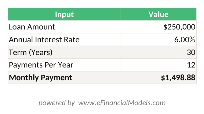
Monthly payment = $1,498.88 via =PMT(6%/12,360,-250000). Period 1 interest = $1,250.00; principal = $248.88. Total interest over 30 years = $289,596.80.

The standard amortization payment formula applied to a $250,000 loan at 6% APR over 30 years yields $1,498.88 per month and $289,597 in total interest.
Four Amortization Scenarios with Downloadable Excel Templates
Amortization applies to four distinct financial contexts, each requiring a different modeling approach. The amortization templates available at EFM cover all four scenarios with pre-built formulas.
Scenario 1: Standard Loan Amortization. Uses PMT, IPMT, and PPMT as described above. Applies to mortgages, term loans, and equipment financing. The schedule fully reconciles to a zero ending balance.
Scenario 2: Intangible Asset Amortization (Straight-Line). Annual amortization expense = (Cost – Residual Value) / Useful Life. For a patent acquired for $500,000 with a 17-year useful life and no residual value: $500,000 / 17 = $29,412 per year. Under IRS Section 197, most acquired intangibles are amortized over 15 years regardless of actual useful life. Software developed internally is typically amortized over 3 to 5 years per FASB ASC 350-40.
Scenario 3: Bond Premium Amortization (Effective Interest Method). When a bond is issued at a premium (above par), the premium is amortized over the bond’s life using the effective interest method. Each period: Interest Expense = Carrying Value × Market Rate; Premium Amortized = Coupon Payment – Interest Expense; New Carrying Value = Prior Carrying Value – Premium Amortized. This method is required under both US GAAP (ASC 835-30) and IFRS (IFRS 9).
Scenario 4: Leasehold Improvement Amortization. Leasehold improvements are amortized over the shorter of the asset’s useful life or the remaining lease term. Under ASC 842, the amortization period must reflect the lease term including renewal options if renewal is reasonably certain. A $120,000 improvement on a 10-year lease with a 5-year remaining term amortizes at $24,000 per year.
For debt amortization modeling across these scenarios, consistent period labeling and a single input block are the two most important structural decisions.
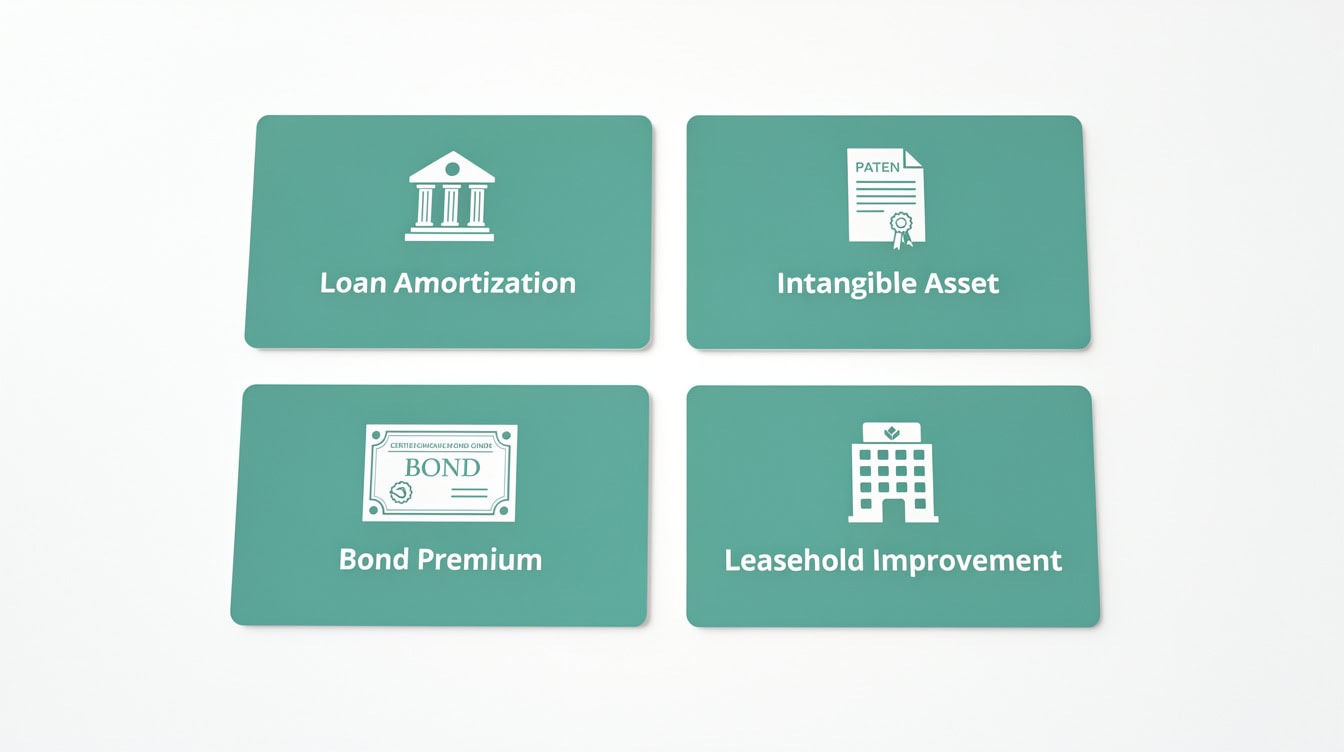
Each of the four amortization scenarios uses a different calculation method and is governed by a different accounting standard.
Amortization vs. Depreciation: Technical Comparison
Amortization and depreciation both allocate asset costs over time, but they apply to different asset classes, use different methods, and carry different tax treatments. Conflating them in a financial model produces errors in both the income statement and the tax schedule. Under IRS MACRS, residential rental property is depreciated over 27.5 years (IRS), while commercial real estate uses a 39-year recovery period — both significantly longer than the 15-year straight-line period mandated by Section 197 for most acquired intangibles.
| Feature | Amortization | Depreciation |
|---|---|---|
| Asset Type | Intangible (patents, goodwill, software) | Tangible (equipment, buildings, vehicles) |
| Common Methods | Straight-line, effective interest | Straight-line, declining balance, MACRS |
| Residual Value | Usually zero | Often non-zero |
| Tax Authority | IRS Section 197 (15-yr rule) | IRS MACRS schedules |
| GAAP Standard | FASB ASC 350 | FASB ASC 360 |
| IFRS Standard | IAS 38 | IAS 16 |
| Abbreviation | AMORT, AMZ, AMTZ | DEPR, D&A (combined) |
| Cash Impact | Non-cash expense | Non-cash expense |
| Balance Sheet | Reduces intangible asset carrying value | Reduces PP&E via accumulated depreciation |
Both appear as non-cash add-backs in the operating section of the cash flow statement. In financial models, D&A (Depreciation and Amortization) is often combined on the income statement but should be split for tax schedule purposes. For business valuation work, EBITDA adds back both D and A, so the split matters for arriving at the correct EBIT figure.
Advanced Non-Linear Amortization Methods and Modeling Techniques
Standard fully-amortizing schedules cover most use cases, but three advanced structures require different modeling approaches: accelerated amortization, balloon payment structures, and variable-rate amortization.
Accelerated Amortization. Front-loads principal repayment to reduce total interest cost. In Excel, model this by adding an “Extra Principal” column to the standard schedule. Each period: Ending Balance = Beginning Balance – Scheduled Principal – Extra Principal. The schedule then terminates early, and you need a MIN() function to cap the final payment at the remaining balance: =MIN(PPMT(…) + Extra_Principal, Beginning_Balance).
Balloon Payment Structures. The loan amortizes on a longer schedule (say 30 years) but becomes due in full at a shorter date (say 7 years). Model this by running the standard 30-year schedule but flagging period 84 (7 × 12) as the balloon date. The balloon payment equals the Ending Balance at period 84 plus the regular period 84 payment. For a $250,000 loan at 6% with a 7-year balloon: the balloon payment at month 84 is approximately $232,160.
Variable-Rate Amortization. Replace the fixed rate cell reference with a lookup table that returns a different rate for each period. Use INDEX/MATCH to pull the applicable rate: =IPMT(INDEX(RateTable,A10)/12, 1, remaining_periods, -B10). Note that with variable rates, you cannot use a single PMT calculation; instead, recalculate the payment each period based on the current rate and remaining balance.
For forecasting purposes, variable-rate models should include a scenario toggle that switches between base, upside, and downside rate paths.

Balloon payment structures amortize on a long schedule but require full repayment at a shorter date, producing a large lump-sum payment at maturity.
Sensitivity Analysis: Rate and Term Changes Impact on Payments
Sensitivity analysis (a technique that shows how output changes when one input varies while others stay fixed) is essential for any amortization model used in credit analysis or investment decisions.
For the $250,000 base case, here is how monthly payment and total interest change across rate and term combinations:
| Rate / Term | 15 Years | 20 Years | 30 Years |
|---|---|---|---|
| 4% Monthly Payment | $1,849.22 | $1,514.99 | $1,193.54 |
| 4% Total Interest | $82,859.60 | $113,597.60 | $179,673.77 |
| 6% Monthly Payment | $2,109.64 | $1,791.86 | $1,498.88 |
| 6% Total Interest | $129,735.20 | $179,646.40 | $289,596.80 |
| 8% Monthly Payment | $2,389.13 | $2,091.10 | $1,834.41 |
| 8% Total Interest | $180,043.40 | $251,864.00 | $410,387.60 |
A 1-percentage-point increase from 6% to 7% on a 30-year, $250,000 loan raises the monthly payment from $1,498.88 to $1,663.26 and increases total interest paid by approximately $59,000 over the loan’s life. This magnitude illustrates why rate sensitivity belongs in every credit model.
In Excel, build this table using a two-variable data table: place the PMT formula in the top-left corner of the table range, list rate values down the left column, and term values across the top row. Then use Data > What-If Analysis > Data Table, setting the row input cell to the term cell and the column input cell to the rate cell.
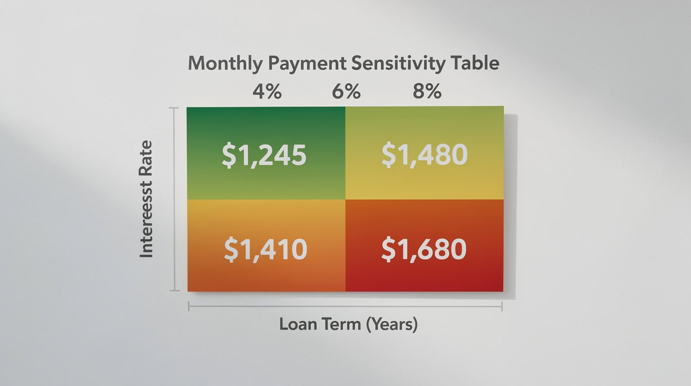
Moving from a 15-year to a 30-year term at 6% reduces the monthly payment by $611 but adds over $159,000 in total interest paid.
Validation Checks and Common Errors in Amortization Modeling
A well-built amortization schedule is self-validating. These are the 5 most common errors practitioners make, and the specific checks that catch them.
Error 1: Using annual rate without dividing by periods. If you enter 6% as the rate argument in PMT without dividing by 12, Excel calculates a monthly payment as if the rate is 6% per month (72% annually). Fix: always use rate/periods_per_year in every PMT, IPMT, and PPMT call.
Error 2: Hardcoding the payment amount. Copying the PMT result as a value rather than keeping the formula breaks the model when inputs change. Fix: always reference the PMT formula cell with a locked absolute reference ($B$6).
Error 3: Final balance not reconciling to zero. Caused by rounding in intermediate calculations. Fix: wrap the final period’s principal payment in a MIN() function: =MIN(PPMT(…), Beginning_Balance). This caps the last principal payment at the actual remaining balance.
Error 4: Mixing beginning-of-period and end-of-period conventions. The type argument in PMT defaults to 0 (end of period). If your lease or bond uses beginning-of-period payments (type=1), every IPMT and PPMT call must also use type=1. Mixing conventions produces incorrect interest splits.
Error 5: Omitting the cumulative interest validation. Add a check row below the schedule: SUM(Interest column) + Loan Amount should equal SUM(Payment column). If it doesn’t, a formula error exists somewhere in the schedule. This single check catches the majority of amortization modeling errors before they reach a client.
For financial planning models that include amortization schedules, these validation checks should be built into the model’s error-checking dashboard alongside balance sheet reconciliation tests.

Building validation checks directly into the amortization model catches formula errors before they reach a reviewer or client.
Frequently Asked Questions
What is the correct abbreviation for amortization in financial models?
The three accepted abbreviations are AMORT, AMZ, and AMTZ. AMORT is the most universally recognized and appears in Big Four working papers, Excel model headers, and GAAP/IFRS footnotes. AMZ is common in Bloomberg terminals and fixed-income software where column space is limited. AMTZ appears in some legacy ERP exports. Never use AMT for amortization because AMT is the established abbreviation for Alternative Minimum Tax under US federal tax law (IRC Section 55), and using it for amortization creates material ambiguity in any tax-adjacent financial model or audit workpaper.
How do I calculate amortization in Excel using PMT, IPMT, and PPMT?
Use three functions together. PMT calculates the fixed periodic payment: =PMT(annual_rate/12, years12, -loan_amount). IPMT calculates the interest portion for a specific period: =IPMT(annual_rate/12, period_number, years12, -loan_amount). PPMT calculates the principal portion: =PPMT(annual_rate/12, period_number, years12, -loan_amount). For a $250,000 loan at 6% over 30 years, PMT returns $1,498.88. In period 1, IPMT returns $1,250.00 and PPMT returns $248.88. Verify your formulas by confirming IPMT + PPMT = PMT for every row in the schedule. Microsoft documents all three functions at support.microsoft.com.
What is the difference between amortization and depreciation for tax purposes?
Amortization applies to intangible assets and is governed by IRS Section 197, which mandates a 15-year amortization period for most acquired intangibles regardless of actual useful life. Depreciation applies to tangible assets and follows IRS MACRS schedules, which vary by asset class: 5 years for computers and vehicles, 7 years for office furniture, 27.5 years for residential rental property, and 39 years for commercial real estate. Both are non-cash expenses that reduce taxable income, but they appear on different lines of the tax return and are governed by different code sections. Mixing them in a financial model produces incorrect effective tax rate calculations.
How does IRS Section 197 affect intangible asset amortization?
IRS Section 197 requires that most intangible assets acquired in a business purchase be amortized over 15 years using the straight-line method, starting from the month of acquisition. This applies to goodwill, customer lists, non-compete agreements, patents, trademarks, and franchises acquired as part of a business purchase. Internally developed intangibles are generally not subject to Section 197 and may be expensed as incurred or capitalized under separate rules. For a $3 million goodwill balance, Section 197 produces annual amortization of $200,000 ($3,000,000 / 15). Note that for financial reporting under GAAP, goodwill is not amortized but is instead tested annually for impairment under FASB ASC 350.
What is the effective interest method for bond premium amortization?
The effective interest method amortizes a bond premium or discount by applying the market interest rate at issuance to the bond’s carrying value each period. Here’s a concrete example: a $1,000,000 bond with a 5% coupon issued when market rates are 4% sells at a premium. Period 1 coupon payment: $1,000,000 × 5% = $50,000. Interest expense at market rate: carrying value × 4% / 2 (for semi-annual) = approximately $21,400. Premium amortized: $50,000 – $21,400 = $28,600. New carrying value: prior carrying value minus $28,600. This method is required under both FASB ASC 835-30 and IFRS 9, and it produces a declining amortization amount each period as the carrying value approaches par.
How do I build a sensitivity table for amortization in Excel?
Use Excel’s two-variable Data Table feature. First, set up your PMT formula in a single cell referencing your rate and term inputs. Then create a table with rate values (4%, 5%, 6%, 7%, 8%) down the left column and term values (15, 20, 30 years) across the top row. Place your PMT formula in the top-left corner of the table range. Select the entire table range including headers, go to Data > What-If Analysis > Data Table, set the row input cell to your term cell and the column input cell to your rate cell, and click OK. Excel populates all 15 combinations instantly. This produces a read-only array formula that updates automatically when you change any input. The table cannot be partially edited; to modify it, you must delete and rebuild.
What validation checks should every amortization schedule include?
Every professional amortization schedule needs at least 4 validation checks. First, the ending balance in the final period must equal zero (or within $0.01 for rounding). Second, the sum of all principal payments must equal the original loan amount. Third, the sum of all payments must equal the sum of all interest plus the original principal: SUM(Payment) = SUM(Interest) + Loan_Amount. Fourth, for each individual row, IPMT + PPMT must equal PMT. Build these as a separate validation block below the schedule, with conditional formatting that turns red when any check fails. These four checks catch the vast majority of formula errors before the model reaches a reviewer or client.
Conclusion
Amortization modeling is a core competency for any finance professional who builds loan schedules, values intangible assets, or prices fixed-income instruments. The abbreviation you use (AMORT or AMZ, never AMT), the Excel functions you apply (PMT, IPMT, PPMT), and the validation checks you build in all determine whether your schedule is audit-ready or error-prone. The $250,000 mortgage example shows that a 30-year loan at 6% costs nearly $290,000 in interest alone, which is exactly the kind of insight that makes a well-built amortization model valuable to decision-makers.
I recommend downloading the EFM Amortization Template Package which includes all four scenarios (loan, intangible asset, bond premium, and leasehold improvement) with pre-built PMT/IPMT/PPMT formulas, a two-variable sensitivity table, and built-in validation checks. It’s the fastest way to move from the concepts in this article to a client-ready deliverable.