0 ITEMS

Multifamily Apartment Financial Model: 15-Hour Shortcut

A multifamily apartment financial model is the analytical engine behind every acquisition, development, and refinancing decision in apartment investing. It projects the income, expenses, debt service, and investor returns for an apartment property over a defined hold period, typically 5 to 10 years, turning market assumptions into the outputs lenders and equity partners use to make go/no-go decisions. This guide shows you exactly how to build one, which of the 8 core modules matter most, and how acquisition, development, and refinancing models differ. It also shows how a purpose-built template cuts build time from 25 to 40 hours down to 8 to 12, saving 15 to 20 hours per deal without sacrificing rigor.
Key Takeaways
- A multifamily apartment financial model must include at least 8 core components: rent roll, unit mix, vacancy/concessions, operating expenses by line item, debt service, capital expenditure reserves, exit valuation, and investor return waterfalls.
- Institutional underwriting clusters around a few hard thresholds: stabilized occupancy of 93 to 95% (modeling above that is a red flag), a minimum Debt Service Coverage Ratio (DSCR) of 1.25x, and loan-to-value (LTV) at or below 80% on conventional agency loans from Fannie Mae and Freddie Mac.
- Replacement reserves for Class B and C multifamily assets typically run $250 to $400 per unit per year, and ignoring this line item is one of the top 5 modeling errors that kill deals.
- A properly structured sensitivity analysis tests at least 4 variables simultaneously: rent growth, expense inflation, exit cap rate, and interest rate, across 3 scenarios (base, upside, downside).
- Templates built for multifamily underwriting cut model-build time from 25 to 40 hours down to 8 to 12 hours, freeing analysts to focus on market judgment rather than formula construction.
- IRR hurdle rates for multifamily investments vary by risk profile: core deals target 7 to 10%, value-add targets 12 to 16%, and opportunistic/development targets 18 to 22%.
What Is a Multifamily Apartment Financial Model?
A multifamily apartment financial model is a structured spreadsheet or software-based tool that projects the income, expenses, debt service, and investor returns for an apartment property over a defined hold period, typically 5 to 10 years. It translates market assumptions and property-specific data into quantified outputs that lenders, equity partners, and operators use to make go/no-go decisions.
The model is not a simple cash flow calculator. It integrates a rent roll (a unit-by-unit schedule of current and projected rents), operating expense forecasts, capital expenditure budgets, financing structures, and exit scenarios into a single connected framework. When one input changes, every output updates automatically. That interconnection is what makes the model a decision-making tool rather than a static spreadsheet.
EFM’s multifamily financial model templates are built specifically for this asset class, with pre-wired rent roll tabs, debt structuring modules, and investor waterfall calculations that match institutional underwriting standards.

All 8 modules must connect: changing one input (e.g., vacancy rate) should automatically update NOI, DSCR, and investor IRR.
Core Components of an Institutional-Grade Multifamily Model
Every institutional-grade multifamily model contains 8 interconnected modules. Missing even one creates blind spots that lenders and equity partners will find during due diligence.
- Rent Roll and Unit Mix: A unit-by-unit schedule showing unit type (studio, 1BR, 2BR, 3BR), square footage, current rent, market rent, lease expiration, and any concessions. This is the foundation of the revenue side.
- Vacancy and Credit Loss: Separate line items for physical vacancy (units not occupied), economic vacancy (occupied but not paying), and concessions (free rent, move-in specials). Blending these into one number hides risk.
- Other Income: Parking, laundry, pet fees, utility reimbursements (RUBS), and ancillary income. For Class A urban assets, other income can represent 8 to 12% of effective gross income.
- Operating Expenses by Category: Management fees, payroll, repairs and maintenance, insurance, property taxes, utilities, marketing, and administrative costs. Each category needs its own growth rate assumption.
- Debt Service Module: Principal and interest calculations for each loan tranche, with the ability to model fixed-rate, floating-rate, interest-only periods, and prepayment penalties.
- Capital Expenditure Reserves: Both immediate capital needs (value-add renovation budgets) and ongoing replacement reserves (roof, HVAC, appliances).
- Exit Valuation: Net Operating Income (NOI) at exit divided by an assumed exit cap rate, less selling costs, to produce net sale proceeds.
- Investor Returns Waterfall: Cash distributions by investor class, preferred return calculations, promote structures, IRR by tranche, and equity multiple.
Acquisition Models vs. Development Models vs. Refinancing Models
These three model types serve different analytical purposes, and using the wrong one for a given situation produces misleading outputs.
An acquisition model starts with an existing rent roll and projects forward from a known income base. The key analytical challenge is underwriting the gap between in-place rents and market rents, and modeling the capital required to close that gap.
A development model (also called a construction model) starts from a blank site or gut-renovation and must project a lease-up period before any stabilized income exists. It carries construction loan interest during the build phase, models absorption rates (the pace at which units lease up), and typically converts to a permanent loan at stabilization. Development models require a Sources and Uses of Capital statement that accounts for land cost, hard construction costs, soft costs (architecture, permits, financing fees), and developer fee.
A refinancing model takes an existing stabilized asset and tests whether current NOI supports a new loan structure, often to return equity to investors. The key output is the new loan amount supportable at a given DSCR, and the resulting cash-out proceeds.
| Model Type | Starting Point | Key Challenge | Primary Output |
|---|---|---|---|
| Acquisition | Existing rent roll | Rent-to-market gap | Levered IRR, equity multiple |
| Development | Empty site or shell | Lease-up absorption | Yield on cost, development spread |
| Refinancing | Stabilized NOI | DSCR at new loan terms | Cash-out proceeds, new returns |
Building the Revenue Side: Rent Roll, Unit Mix, and Market Rent Projections
The revenue side of a multifamily model starts with the rent roll and builds outward to effective gross income. Gross Potential Rent (GPR) is the maximum rent the property could collect if every unit were occupied at market rent with no concessions. From GPR, you subtract vacancy, concessions, and credit loss to arrive at Effective Gross Income (EGI).
Here’s the math for a 100-unit property:
- Gross Potential Rent: 100 units x $1,800/month x 12 months = $2,160,000
- Less Physical Vacancy (5%): ($108,000)
- Less Concessions (1%): ($21,600)
- Less Credit Loss (0.5%): ($10,800)
- Effective Gross Income: $2,019,600
- Plus Other Income (parking, laundry, etc.): $48,000
- Total Effective Gross Income: $2,067,600
Rent growth assumptions must be differentiated by unit type and lease term. A model that applies a single annual rent growth rate to the entire rent roll ignores the reality that studios and 3-bedroom units respond differently to market conditions. Institutional underwriters typically apply market-specific rent growth forecasts from sources such as CoStar or CBRE Research, rather than using a single national average.
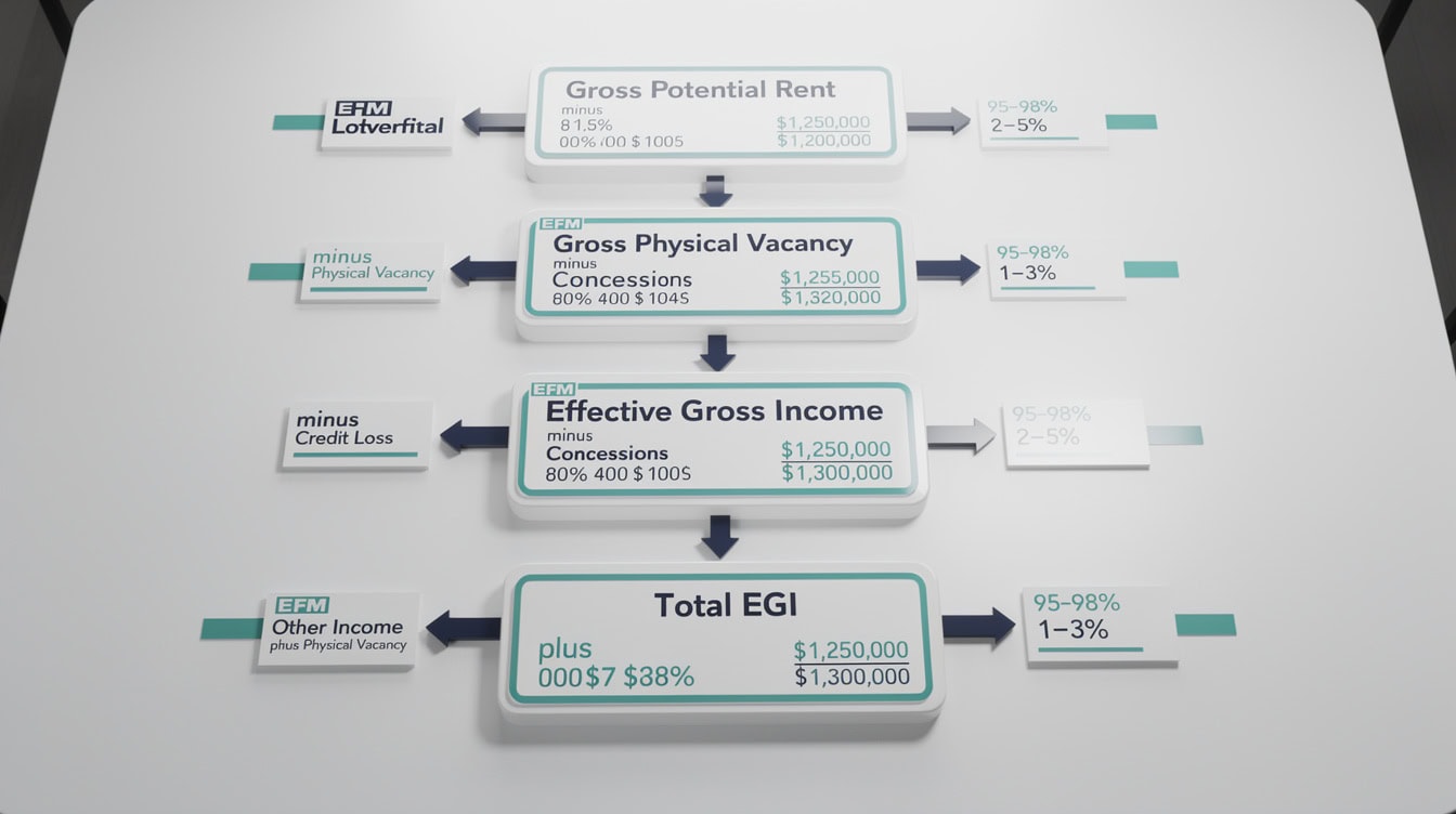
Separating physical vacancy, concessions, and credit loss into distinct line items allows independent stress-testing of each revenue risk.
Operating Expense Modeling: Line-Item Detail That Matters
Operating expenses in a multifamily model must be projected at the line-item level, not as a single percentage of revenue. The expense ratio (total operating expenses divided by effective gross income) varies significantly by asset class and geography.
Class A urban high-rise properties typically carry expense ratios of 45 to 55% due to higher payroll, amenity costs, and property taxes. Class B suburban garden-style properties typically run 38 to 48%. Class C workforce housing can run 50 to 60% because deferred maintenance and higher turnover inflate repair costs. Property taxes represent the single largest operating expense category for most multifamily assets, averaging 25 to 30% of total operating expenses in high-tax states, according to National Apartment Association research on rental housing operating costs.
Property tax reassessment is a critical modeling variable that many analysts underestimate. In many jurisdictions, a sale triggers a reassessment to the purchase price. A model that carries forward the seller’s current tax bill without adjusting for reassessment will overstate NOI by a material amount. For a $20 million acquisition in a state with a 1.2% effective tax rate, the difference between the seller’s assessed value and the purchase price could add $60,000 to $120,000 in annual property tax expense.

Class C assets often carry higher expense ratios than Class A despite lower rents, because deferred maintenance and turnover costs compound over time.
Debt Structures and Financing Scenarios in Multifamily Models
Multifamily properties have access to the broadest range of debt financing of any commercial real estate asset class, and the model must accommodate multiple structures simultaneously.
Agency debt from Fannie Mae and Freddie Mac dominates the multifamily lending market. Federal Housing Finance Agency data on Enterprise multifamily loan purchases shows that Fannie Mae and Freddie Mac together purchased or guaranteed over $140 billion in multifamily mortgage loans in 2023. Agency loans typically offer 10-year fixed terms with 30-year amortization, LTV ratios up to 80%, and DSCR minimums of 1.25x. Interest-only periods of 2 to 5 years are common on agency loans for stabilized assets.
Bank balance sheet loans, CMBS (Commercial Mortgage-Backed Securities) loans, bridge loans for value-add acquisitions, and construction loans for development each have different parameters that the model must capture. A robust multifamily model includes a financing assumptions tab where the user can toggle between loan types and see the impact on cash flow and returns in real time.
| Loan Type | Typical LTV | Min DSCR | Term | Best For |
|---|---|---|---|---|
| Agency (Fannie/Freddie) | Up to 80% | 1.25x | 10 years | Stabilized assets |
| Bank Balance Sheet | 65-75% | 1.20x | 3-7 years | Smaller deals |
| Bridge Loan | 70-80% | 1.05-1.15x | 1-3 years | Value-add/lease-up |
| Construction Loan | 60-70% of cost | Interest only | 18-36 months | Ground-up development |
| CMBS | 70-75% | 1.25x | 5-10 years | Larger stabilized |
Capital Expenditures and Reserve Planning
Capital expenditure modeling in multifamily goes beyond a simple per-unit reserve. It requires separating immediate capital needs from ongoing replacement reserves, and both from value-add renovation budgets.
Replacement reserves cover the eventual replacement of major building systems: roofs, HVAC units, elevators, parking surfaces, and appliances. The Institute of Real Estate Management recommends replacement reserves of $200 to $300 per unit per year for newer Class A assets, and $300 to $500 per unit per year for older Class B and C properties. Lenders often require a minimum reserve deposit as a condition of the loan, and the model must reflect this as a cash outflow separate from operating expenses.
For value-add repositioning, the renovation budget must be modeled unit by unit or by renovation tier (light, medium, heavy), with a clear assumption about the rent premium each tier achieves and the payback period. A $12,000 per-unit renovation that generates a $150/month rent premium has a payback period of 80 months (6.7 years), which must be weighed against the hold period and exit cap rate assumptions.
Modeling Lease-Up, Stabilization, and Value-Add Repositioning
Lease-up modeling is the most complex revenue-side challenge in multifamily development and value-add acquisition models. Stabilization (the point at which a property reaches its target occupancy and rent levels) rarely happens overnight, and the model must reflect the absorption curve realistically.
For new construction in a primary market, typical absorption rates run 15 to 25 units per month for a well-located, well-priced property. A 200-unit building at 20 units per month takes 10 months to reach 100% occupancy, but the model should target 93 to 95% stabilized occupancy, not 100%. During lease-up, concessions (free rent, waived fees) reduce effective rent, and the model must capture both the concession cost and the burn-off period as the property stabilizes.
For value-add repositioning, the model must layer in renovation timing (how many units are taken offline each month for renovation), the rent premium achieved on renovated units, and the transition period between the old rent roll and the stabilized renovated rent roll. Analysts who model value-add as a simple step-change from current rents to market rents on day one will overstate early-period cash flow and understate the capital required during the transition.
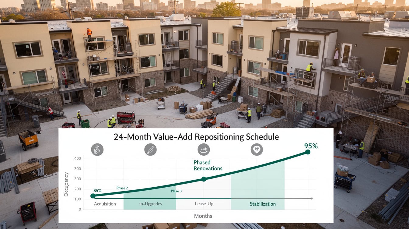
A phased renovation schedule prevents taking too many units offline simultaneously, protecting cash flow during the repositioning period.
Returns Analysis: IRR, Equity Multiple, Cash-on-Cash, and Yield on Cost
A multifamily financial model produces four primary return metrics, each serving a different analytical purpose.
IRR (Internal Rate of Return) is the discount rate that makes the net present value of all cash flows equal to zero. It accounts for the time value of money and is the standard metric for comparing investments with different hold periods. For multifamily, IRR is calculated on levered cash flows (after debt service) from the investor’s perspective.
Equity Multiple is total cash returned to equity divided by total equity invested. A 2.0x equity multiple means the investor doubled their money, regardless of how long it took. IRR and equity multiple together tell the full story: a 20% IRR over 2 years and a 15% IRR over 7 years have very different equity multiples.
Cash-on-Cash Return is annual cash flow after debt service divided by total equity invested. It measures current income yield and is particularly important for investors who need current distributions rather than back-end appreciation.
Yield on Cost is stabilized NOI divided by total project cost (acquisition plus renovation or construction). It measures the return on the total capital deployed and is used to evaluate whether a development or value-add project creates value relative to the market cap rate.
According to data from CBRE’s U.S. Cap Rate Survey, multifamily cap rates in primary markets ranged from 4.5 to 5.5% for Class A assets and 5.5 to 6.5% for Class B assets as of late 2024. A development project that achieves a 6.5% yield on cost in a 5.0% cap rate market has created a 150-basis-point development spread, representing meaningful value creation.
You can explore pre-built DCF model templates and 5-year financial projection models at EFM to see how these return metrics are wired together in practice.
Sensitivity Analysis and Scenario Planning for Risk Management
Sensitivity analysis tests how the model’s key outputs (IRR, equity multiple, DSCR) change when input assumptions change. Every multifamily model must include sensitivity tables as a core deliverable, not an afterthought.
The 4 variables that matter most in multifamily sensitivity analysis are: exit cap rate, rent growth, expense inflation, and interest rate (for floating-rate debt). A two-variable sensitivity table showing IRR across a range of exit cap rates and rent growth assumptions is the minimum standard for institutional underwriting.
| Exit Cap Rate / Rent Growth | 1% | 2% | 3% | 4% |
|---|---|---|---|---|
| 4.50% | 18.2% | 20.1% | 22.3% | 24.6% |
| 5.00% | 14.8% | 16.5% | 18.4% | 20.5% |
| 5.50% | 11.3% | 13.0% | 14.8% | 16.8% |
| 6.00% | 7.9% | 9.5% | 11.2% | 13.1% |
| 6.50% | 4.4% | 6.0% | 7.6% | 9.4% |
This table shows levered IRR for a hypothetical 100-unit value-add acquisition. The deal works at a 5.0% exit cap with 2% rent growth (16.5% IRR) but fails to meet a 12% hurdle at a 6.0% exit cap with 1% rent growth (7.9% IRR). Scenario planning goes further, combining multiple variable changes into named scenarios (base, upside, downside, stress) that tell a coherent story about the range of outcomes.
Common Multifamily Modeling Mistakes That Kill Deals
Modeling errors in multifamily underwriting fall into 5 recurring categories. Each one has a specific fix.
1. Ignoring Property Tax Reassessment: The fix is to model property taxes based on the purchase price multiplied by the local effective tax rate, not the seller’s current tax bill. Build in a 12 to 24-month lag for reassessment timing.
2. Omitting Replacement Reserves: Many first-time models treat replacement reserves as optional. They are not. Lenders require them, and omitting them overstates cash flow. Use $250 to $400 per unit per year as a starting point and adjust for asset age and condition.
3. Overly Aggressive Rent Growth: Underwriting 4 to 5% annual rent growth in a market where historical rent growth has averaged 2 to 3% is a common error. The U.S. Bureau of Labor Statistics Consumer Price Index shelter series shows the shelter component of CPI (a proxy for rent inflation) averaged 5.4% annually from 2021 to 2023. However, long-run averages are closer to 3%. Model rent growth conservatively in the base case and reserve optimism for the upside scenario.
4. Blending Vacancy into a Single Number: Physical vacancy, economic vacancy, and concessions are three distinct phenomena. Blending them hides the source of revenue leakage and makes it impossible to stress-test each component independently.
5. Mismodeling Interest-Only Periods: When a loan has a 3-year interest-only period followed by amortization, the model must switch from interest-only payments to fully amortizing payments at the right month. Getting this wrong overstates cash flow in years 4 and beyond and understates the DSCR at the point of amortization.
How Templates Accelerate Underwriting Without Sacrificing Rigor
A well-built multifamily apartment financial model template saves 15 to 20 hours per deal by eliminating the time spent building formulas, formatting outputs, and wiring modules together. An analyst building a multifamily model from scratch typically spends 25 to 40 hours on the first version. A template reduces that to 8 to 12 hours of data entry and assumption-setting.
The time savings come from pre-built infrastructure: rent roll tabs with automatic unit mix summaries, debt service schedules that update when loan terms change, sensitivity tables that recalculate automatically, and investor waterfall calculations that handle preferred returns and promote structures without manual intervention.
What templates cannot replace is analytical judgment: the decision about what rent growth rate to use, whether the market supports the exit cap rate assumption, and whether the renovation budget is realistic. Templates handle the math; the analyst handles the market knowledge.
EFM’s financial model templates for real estate include multifamily-specific models with built-in rent roll analysis, three-statement integration, and investor reporting outputs. For development projects, EFM’s financial projections templates include construction draw schedules and lease-up absorption modeling.

A purpose-built multifamily template cuts model-build time from 25-40 hours to 8-12 hours, freeing analysts to focus on market judgment.
Frequently Asked Questions About Multifamily Financial Models
What should a multifamily apartment financial model template include at minimum?
A multifamily apartment financial model template must include, at minimum, a rent roll tab with unit-by-unit detail, a vacancy and concessions schedule, an operating expense forecast with at least 8 line items, a debt service module that handles both fixed and floating rate loans, a capital expenditure reserve schedule, an exit valuation using the income capitalization approach (NOI divided by cap rate), and an investor returns summary showing IRR, equity multiple, and cash-on-cash return. Templates that combine these into a single connected workbook, where changing one assumption updates all outputs, are the standard for institutional underwriting. EFM’s multifamily templates include all of these components plus a sensitivity analysis dashboard and a distribution waterfall for equity partners.
How do I model the lease-up period for a new multifamily development?
Modeling lease-up requires three inputs: the absorption rate (units leased per month), the concession package (typically 4 to 8 weeks of free rent in competitive markets), and the target stabilized occupancy (typically 93 to 95%). Start with zero occupancy at certificate of occupancy, add the monthly absorption rate, and apply concessions to the first 6 to 12 months of leases. The model should show month-by-month occupancy, effective rent per unit (after concessions), and total effective gross income until the property reaches stabilization. For a 150-unit building absorbing 18 units per month, stabilization takes approximately 8 to 9 months. During that period, the construction loan is typically still outstanding, and the model must capture the interest carry on the construction loan as a cost.
What DSCR do lenders require for multifamily loans?
Debt Service Coverage Ratio (DSCR) is Net Operating Income divided by annual debt service (principal plus interest). Agency lenders (Fannie Mae and Freddie Mac) require a minimum DSCR of 1.25x for most conventional multifamily loans, meaning NOI must be at least 25% higher than the annual debt service payment. Some agency programs for affordable housing or small balance loans allow DSCRs as low as 1.15x. Bank balance sheet lenders typically require 1.20x to 1.25x. Bridge lenders for value-add acquisitions may accept 1.05x to 1.15x during the lease-up period, with a covenant to reach 1.25x at stabilization. Your model must calculate DSCR for every year of the hold period, not just at acquisition.
What is a realistic IRR target for a multifamily value-add investment?
IRR targets for multifamily investments depend on the risk profile and hold period. Core multifamily investments (stabilized, Class A, primary markets) typically target levered IRRs of 7 to 10%. Value-add investments (Class B or C assets requiring renovation and repositioning) typically target 12 to 16% levered IRR. Opportunistic or ground-up development deals target 18 to 22% or higher to compensate for construction and lease-up risk. These hurdle rates are set by the equity partner or fund manager and represent the minimum acceptable return given the risk taken. A model that shows a 14% IRR on a value-add deal in a primary market is generally considered attractive; the same 14% IRR on a ground-up development in a secondary market would likely be below the hurdle rate for most institutional equity partners.
How do I model a preferred return and promote structure in a multifamily waterfall?
A waterfall distribution model (also called a waterfall structure) defines the order in which cash flows are distributed between the operating partner (GP) and the equity investors (LPs). A typical structure works as follows: first, return of capital to all investors; second, a preferred return (commonly 6 to 8% annually) paid to LPs before the GP receives any promote; third, a catch-up provision where the GP receives a larger share until they reach their target promote percentage; fourth, remaining cash split according to the agreed promote structure (commonly 70/30 or 80/20 LP/GP). The model must calculate these distributions for both current cash flow (annual distributions) and the exit proceeds. IRR is calculated separately for the LP and GP to show each party’s return. EFM’s waterfall distribution models handle multi-tier promote structures with automatic IRR calculations by investor class.
What is the difference between a Class A, B, and C multifamily model?
Class A, B, and C multifamily assets require different modeling assumptions across revenue, expenses, and capital expenditures. Class A assets (built within the last 10 to 15 years, high-end finishes, premium amenities) carry lower expense ratios on repairs and maintenance but higher payroll and amenity costs, and they command the lowest cap rates (highest valuations). Class B assets (built 15 to 30 years ago, moderate finishes) are the most common value-add target and require renovation budgets of $8,000 to $20,000 per unit to achieve market rents. Class C assets (older vintage, workforce housing) carry the highest expense ratios (50 to 60% of EGI), the highest replacement reserve requirements ($350 to $500 per unit per year), and the highest cap rates. A model built for Class A assumptions applied to a Class C asset will systematically overstate NOI and understate capital requirements, producing an IRR that looks attractive but reflects modeling error rather than real returns.
How long does it take to build a multifamily financial model from scratch vs. using a template?
Building a multifamily financial model from scratch takes an experienced analyst 25 to 40 hours for a complete institutional-grade model, including rent roll, debt service, sensitivity analysis, and investor waterfall. A junior analyst may take 40 to 60 hours. Using a purpose-built template reduces that to 8 to 12 hours of data entry, assumption-setting, and market research. The time savings are largest on the structural elements (formula construction, formatting, waterfall logic) and smallest on the judgment-intensive elements (market rent research, expense benchmarking, cap rate selection). For firms underwriting 20 to 30 deals per year, the cumulative time savings from using templates can exceed 300 to 600 analyst hours annually.
Conclusion
A multifamily apartment financial model is not a commodity spreadsheet. It is a decision-making system that integrates market data, property-specific assumptions, financing structures, and investor return requirements into a single analytical framework. The difference between a model that closes deals and one that kills them often comes down to 5 specific errors: ignoring property tax reassessment, omitting replacement reserves, applying aggressive rent growth, blending vacancy components, and mismodeling interest-only periods.
Templates solve the structural problem. Analytical judgment solves the market problem. You need both.
I recommend downloading EFM’s institutional-grade Multifamily Apartment Financial Model Template to start underwriting your next deal with a pre-built rent roll, debt structuring module, sensitivity dashboard, and investor waterfall, saving 15 to 20 hours on your first deal alone.