0 ITEMS

Calculate Revenue in Excel: Formulas That Actually Work
The fastest way to calculate revenue in Excel is =SUMPRODUCT(units_range, price_range), but real business revenue rarely fits a single formula.
Key Takeaways
- The SUMPRODUCT function calculates multi-product revenue in 1 formula, replacing dozens of row-by-row multiplications.
- Named ranges cut formula errors by making cell references self-documenting, for example
=Units_Sold*Unit_Priceinstead of=B2*C2. - SUMIFS lets you slice revenue by region, product, or date with a single formula, no pivot table required.
- A period-over-period growth rate formula
=(Current-Prior)/Priortakes 5 seconds to build and is the foundation of every revenue dashboard. - Excel’s FORECAST.ETS function handles seasonality automatically, producing more accurate projections than a simple linear trend.
- Circular reference errors and #VALUE! errors account for the majority of revenue miscalculations in spreadsheet models, and both have straightforward fixes.
- Structuring your workbook with separate Input, Calculation, and Output sheets reduces audit time and prevents accidental formula overwrites.
Understanding Revenue Calculation Fundamentals in Excel
Revenue (also called top-line income) is the total money a business earns from selling goods or services before any costs are deducted. In Excel, every revenue calculation reduces to one core operation: multiplying quantity by price, then aggregating across products, time periods, or customer segments. Getting that structure right before writing a single formula saves hours of troubleshooting later.
Research collected by the European Spreadsheet Risk Interest Group (EuSpRIG) finds that more than 90% of spreadsheets contain errors, and that around half of the spreadsheets used operationally in large businesses carry material defects. Revenue models sit at the riskier end of that range because they combine multiple data sources and formula types.
That statistic alone makes a disciplined approach to Excel revenue calculation worth the investment.
Before building any formula, set up three worksheet tabs: Inputs (raw data and assumptions), Calculations (formulas only, no hard-coded numbers), and Outputs (summary tables and charts). This separation is the single most effective structural practice in financial modeling.

Separating inputs from formulas and outputs is the single most effective structural practice in financial modeling.
Essential Excel Formulas for Single-Product Revenue Calculation
For a single product, revenue equals units sold multiplied by price per unit. In Excel, place units in column A and price in column B, then enter =A2*B2 in column C. To total a column of revenues, wrap it in SUM: =SUM(C2:C100).
Here’s the math for a simple example:
- Units sold: 500
- Price per unit: $40
- Revenue:
=500*40= $20,000
When your data lives in a formatted Excel Table (Insert > Table), the formula becomes =[@Units]*[@Price] and auto-fills to every new row. Microsoft’s guidance on structured references explains that these names adjust automatically whenever you add or remove data from the table, which eliminates the most common range-expansion error in revenue models.
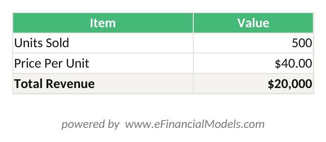
Total Revenue = Units Sold × Price Per Unit. The formula in B4 references B2 and B3 so the result updates automatically when inputs change.
Multi-Product Revenue Models Using SUMPRODUCT and Array Formulas
SUMPRODUCT is the workhorse formula for multi-product revenue. It multiplies corresponding values in two or more arrays (a set of values treated as a group) and sums the results, all in one step. The syntax is =SUMPRODUCT(array1, array2).
Worked example with 3 products:
| Product | Units | Price | Revenue |
|---|---|---|---|
| A | 200 | $15 | $3,000 |
| B | 350 | $22 | $7,700 |
| C | 120 | $45 | $5,400 |
| Total | $16,100 |
Instead of summing column D, use: =SUMPRODUCT(B2:B4, C2:C4)
Here’s the calculation step by step:
- Multiply each pair: 200×15=3,000 | 350×22=7,700 | 120×45=5,400
- Sum the products: 3,000 + 7,700 + 5,400 = $16,100
SUMPRODUCT also accepts conditions. To calculate revenue only for products priced above $20: =SUMPRODUCT((C2:C4>20)*B2:B4*C2:C4). The condition (C2:C4>20) returns an array of 1s and 0s (boolean logic, meaning true/false values converted to numbers), which filters the multiplication.
For revenue projections across many product lines, SUMPRODUCT scales without modification as you add rows to your table.
Handling Complex Revenue Scenarios: Discounts, Returns, and Subscriptions
Real revenue models must account for price adjustments, customer returns, and recurring billing cycles. Each scenario requires a specific formula approach.
Discounts: Net revenue after a 10% discount on a $20,000 gross figure:=(Units*Price)*(1-Discount_Rate) = =(500*40)*(1-0.10) = $18,000
Returns: Subtract returned units before multiplying:=(Units_Sold - Units_Returned)*Price = =(500-30)*40 = $18,800
Subscription (MRR to ARR): Monthly Recurring Revenue (MRR) is the predictable monthly revenue from active subscribers. Annual Recurring Revenue (ARR) is MRR multiplied by 12. If you have 300 subscribers paying $99/month:
- MRR =
=300*99= $29,700 - ARR =
=MRR*12= $356,400
For SaaS businesses tracking Monthly Recurring Revenue and Annual Recurring Revenue, building these as named ranges (Formulas > Define Name) makes the model readable and auditable.
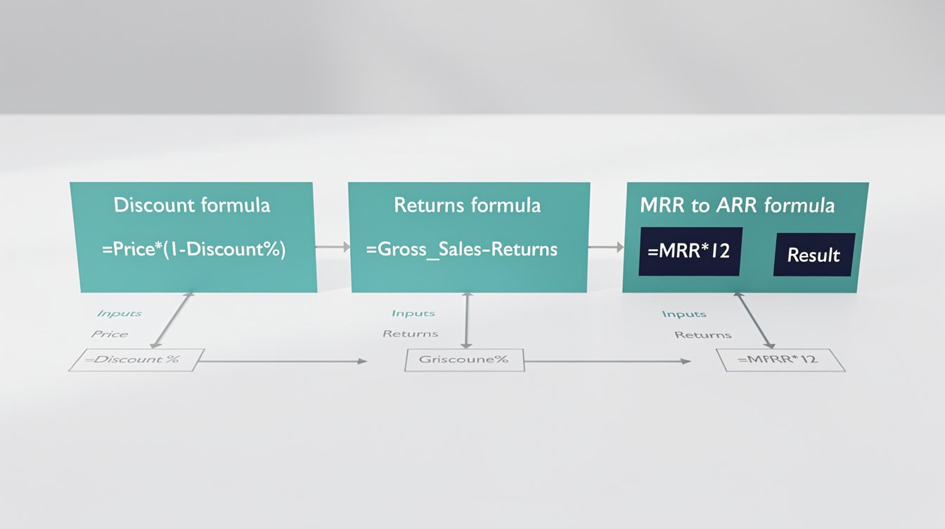
Discount, return, and subscription formulas each require a distinct structure to produce accurate net revenue figures.
Building Dynamic Revenue Calculators with Named Ranges and Data Validation
A dynamic revenue calculator updates every output automatically when you change a single input. Named ranges and data validation are the two tools that make this possible.
Named ranges assign a label to a cell or range. Instead of =B2*C2, you write =Units_Sold*Unit_Price. Microsoft’s walkthrough on defining and using names in formulas sets out the steps: select the cell, go to Formulas > Define Name, and type the label. The accompanying naming syntax rules allow up to 255 characters per name and forbid spaces, so use underscores or periods as separators.
Data validation restricts inputs to valid ranges, preventing a user from entering a negative price or a text string where a number belongs. Set it via Data > Data Validation > Whole Number or Decimal, then specify minimum and maximum values.
Combine both: create a dropdown list of product names using data validation, then use VLOOKUP or XLOOKUP to pull the corresponding price automatically. The formula =XLOOKUP(A2, ProductTableName, ProductTablePrice) returns the price for whatever product the user selects, making the entire revenue model respond to a single dropdown change.
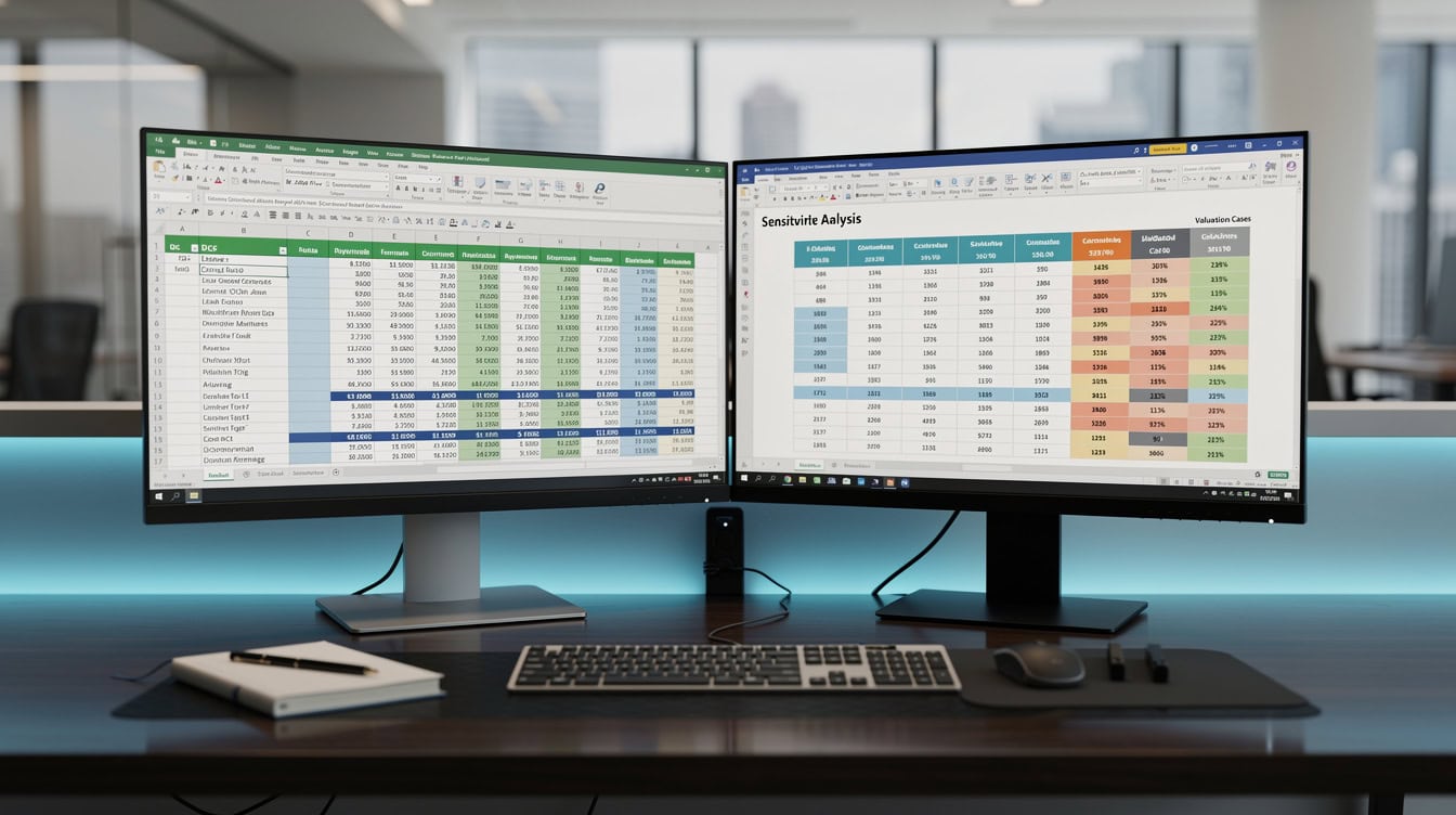
Combining data validation dropdowns with XLOOKUP creates a revenue calculator that updates with a single selection.
Revenue Growth Analysis: Period-over-Period and Year-over-Year Calculations
Revenue growth rate measures how fast top-line income is expanding between two periods. The formula is straightforward: =(Current_Period - Prior_Period) / Prior_Period.
Example: Q1 revenue = $120,000; Q2 revenue = $138,000
- Growth rate =
=(138000-120000)/120000= 15%
For year-over-year (YoY) analysis across a full dataset, apply this formula across a column and format as percentage. To calculate a compound annual growth rate (CAGR), which smooths out year-to-year volatility, use:=(End_Value/Start_Value)^(1/Years)-1
If revenue grew from $500,000 to $950,000 over 4 years:=(950000/500000)^(1/4)-1 = 17.4% CAGR
For cost calculation and margin analysis alongside these growth figures, keep a parallel column tracking cost of goods sold so gross margin trends are visible in the same view.
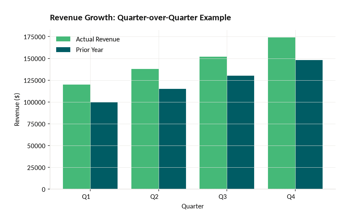
Quarter-over-quarter revenue growth calculated using =(Current-Prior)/Prior. Q4 shows 17.6% YoY growth in this example.
Common Revenue Formula Errors and How to Fix Them
Five formula errors cause the vast majority of revenue calculation mistakes. Each has a specific fix.
| Error | Cause | Fix |
|---|---|---|
| #VALUE! | Text in a numeric range | Use ISNUMBER() to audit; clean data with VALUE() |
| #REF! | Deleted row/column breaks a reference | Rebuild the reference; use Table references to prevent recurrence |
| #DIV/0! | Dividing by zero (e.g., prior period = 0) | Wrap in IFERROR: =IFERROR(A2/B2,0) |
| Circular reference | Formula references its own cell | Enable iterative calculation or restructure the formula chain |
| Wrong range | SUM includes header row | Always start range at row 2, or use Table references |
Circular reference (a formula that refers back to itself, creating an infinite loop) is the trickiest. Excel flags it in the status bar. The fix is almost always to move the formula to a separate cell that doesn’t feed back into its own inputs. If you genuinely need iterative calculation, enable it under File > Options > Formulas > Enable iterative calculation, but document this clearly in your model.
To validate totals, use a cross-check formula: =SUM(Revenue_Column)-SUM(Units_Column*Price_Column). This should always equal zero. If it doesn’t, a data entry error or formula mismatch exists somewhere in the model.
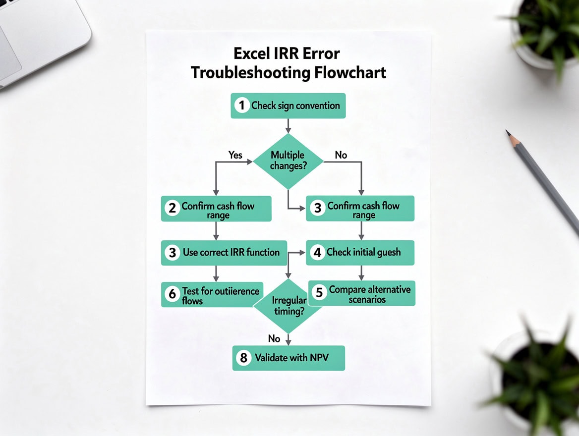
IFERROR wrapping and structured Table references eliminate the most common revenue formula errors before they reach a report.
Revenue Forecasting with Excel Trend and Regression Functions
Excel offers three practical forecasting approaches for revenue: linear trend, moving average, and exponential smoothing.
FORECAST.LINEAR projects a future value based on a straight-line trend through historical data: =FORECAST.LINEAR(future_x, known_ys, known_xs). If your x-axis is month numbers 1-12 and y-axis is monthly revenue, this formula extrapolates the trend.
FORECAST.ETS handles seasonality automatically. Microsoft’s FORECAST.ETS function reference describes it as predicting future values using the AAA version of the Exponential Smoothing (ETS) algorithm, which weights recent data more heavily while accounting for repeating seasonal patterns, and lists the function for desktop Excel 2019 and later as well as Microsoft 365.
For retail or hospitality businesses with clear seasonal peaks, FORECAST.ETS consistently outperforms a simple linear projection.
Moving average smooths short-term fluctuations. A 3-month moving average for month 4 is: =AVERAGE(B2:B4). Drag the formula down to apply it across the full dataset.
For Excel-based financial models that need to present forecasts to stakeholders, pair the FORECAST.ETS output with a confidence interval using the FORECAST.ETS.CONFINT function to show the range of likely outcomes, not just a single point estimate.

FORECAST.ETS accounts for seasonal patterns automatically, producing more reliable projections than a linear trend line.
Creating Revenue Dashboards and Executive Reports
A revenue dashboard connects your calculation sheet to visual summaries that executives can read in 30 seconds. The three components are pivot tables, charts, and conditional formatting.
Pivot tables summarize revenue by any dimension (product, region, month) without changing the underlying data. Select your revenue table, go to Insert > PivotTable, and drag Revenue to Values, Month to Rows, and Product to Columns. The pivot table recalculates instantly when source data updates.
Charts: A clustered bar chart works best for comparing revenue across products. A line chart shows trend over time. Right-click any pivot table and select PivotChart to link the two directly.
Conditional formatting highlights revenue cells that fall below target. Select the revenue column, go to Home > Conditional Formatting > Highlight Cell Rules > Less Than, enter your target, and choose a red fill. This creates an instant visual alert without any additional formula work.
For a complete dashboard structure, place the pivot table on the left, the chart on the right, and a KPI summary row at the top showing total revenue, growth rate, and variance to budget. This layout matches the reading pattern most executives use: headline numbers first, detail second.

A three-component dashboard layout (KPIs top, pivot table left, chart right) matches the reading pattern most executives use.
Best Practices for Revenue Model Documentation and Audit Trails
A revenue model that only its creator can understand is a liability. Three practices make models auditable by anyone.
Document assumptions inline: Use Excel comments (right-click > Insert Comment) or a dedicated Assumptions tab to record the source and rationale for every input. Note the date, the source (for example, “Sales forecast from CRM export, 2024-Q3”), and the owner.
Protect formula cells: Select all formula cells, go to Home > Format > Lock Cell, then protect the sheet via Review > Protect Sheet. This prevents accidental overwrites while leaving input cells editable.
Version control: Save dated copies (Revenue_Model_2024-10-01.xlsx) before major changes. For team environments, use SharePoint or OneDrive version history, which retains up to 500 versions of a file automatically.
Color-coding inputs vs. formulas is a widely used convention: blue font for hard-coded inputs, black font for formulas. This visual distinction lets any reviewer immediately identify where to change assumptions without touching formula logic.
Frequently Asked Questions
What is the simplest formula to calculate revenue in Excel?
The simplest revenue formula is =A2*B2, where A2 contains units sold and B2 contains the price per unit. For a single product with one price, this is all you need. To total revenue across multiple rows, wrap it in SUM: =SUM(C2:C100) where column C contains the individual row revenues. If you want to skip the helper column entirely, use SUMPRODUCT: =SUMPRODUCT(A2:A100, B2:B100). This single formula multiplies each unit-price pair and sums the results in one step, making it the preferred approach for models with more than a handful of products. Always format the result cell as Currency (Ctrl+1 > Number > Currency) so the output reads clearly in reports.
How do I calculate revenue with discounts in Excel?
To calculate net revenue after a discount, use the formula =(Units*Price)*(1-Discount_Rate). For example, if cell A2 holds 500 units, B2 holds $40 price, and C2 holds a 10% discount rate, the formula is =(A2*B2)*(1-C2), which returns $18,000. For tiered discounts where the rate changes based on volume, use a nested IF or VLOOKUP to pull the correct discount rate from a lookup table before applying it. Store discount rates in a separate Assumptions tab so they’re easy to update without touching the formula structure. This approach also makes the discount assumption visible during audits.
What is the difference between SUMIF and SUMPRODUCT for revenue calculation?
SUMIF adds values in a range that meet a single condition, for example =SUMIF(Region, "North", Revenue) totals revenue only for the North region. SUMPRODUCT multiplies arrays together and sums the result, making it ideal for calculating total revenue across multiple products in one step: =SUMPRODUCT(Units, Price). SUMPRODUCT also handles multiple conditions without needing SUMIFS: =SUMPRODUCT((Region="North")*(Product="A")*Units*Price). Use SUMIF when you need a conditional total of existing revenue values. Use SUMPRODUCT when you need to calculate revenue from component inputs (units and price) while optionally filtering by one or more criteria. SUMPRODUCT is generally more flexible but slightly slower on very large datasets (100,000+ rows).
How do I calculate year-over-year revenue growth in Excel?
Year-over-year (YoY) revenue growth measures the percentage change between the same period in two consecutive years. The formula is =(Current_Year - Prior_Year) / Prior_Year. If 2023 revenue was $1,200,000 and 2024 revenue is $1,440,000, the formula returns =(1440000-1200000)/1200000 = 20%. Format the result as a percentage (Ctrl+Shift+%). To calculate compound annual growth rate (CAGR) over multiple years, use =(End_Value/Start_Value)^(1/Number_of_Years)-1. For a revenue model that grew from $500,000 to $950,000 over 4 years, CAGR = =(950000/500000)^(0.25)-1 = 17.4%. CAGR is the preferred metric for investor presentations because it smooths out year-to-year volatility.
How do I handle #DIV/0! errors in revenue growth formulas?
A #DIV/0! error appears when your growth formula divides by a prior-period value of zero, which happens when a product launched mid-year or a revenue stream is new. Wrap the formula in IFERROR to return a clean result: =IFERROR((Current-Prior)/Prior, "N/A"). You can also return 0 or a specific text string depending on how the model will be used. For dashboards, “N/A” is clearer than 0 because it signals a genuine data gap rather than flat growth. A more robust approach uses an IF check: =IF(Prior=0, "New", (Current-Prior)/Prior). This labels new revenue streams explicitly, which is more informative for stakeholders reviewing the report than a blank cell or error code.
Can Excel handle subscription and recurring revenue models?
Yes. For subscription businesses, the key metrics are MRR (Monthly Recurring Revenue) and ARR (Annual Recurring Revenue). MRR = active subscribers multiplied by average monthly price: =Subscribers*Monthly_Price. ARR = =MRR*12. To model churn (the rate at which subscribers cancel), apply: =Prior_Subscribers*(1-Churn_Rate)+New_Subscribers. For a SaaS business with 1,000 subscribers, a 2% monthly churn rate, and 50 new subscribers per month, next month’s subscriber count = =1000*(1-0.02)+50 = 1,030. Build this formula across 12 rows to project a full year of subscriber counts, then multiply by price to get monthly revenue. The SaaS Financial Model Excel Template at EFM includes this structure pre-built.
What is the best way to structure an Excel revenue model for a multi-product business?
The best structure separates inputs, calculations, and outputs across three tabs. On the Inputs tab, list every product with its unit price, expected volume, and any discount or return rate. On the Calculations tab, use SUMPRODUCT or structured Table references to compute revenue by product and period. On the Outputs tab, build a pivot table or summary table that pulls from the Calculations tab. Never mix hard-coded numbers with formulas in the same cell. Use named ranges for all key inputs so formulas read as =Units_ProductA * Price_ProductA rather than =B7*C7. This structure means any team member can update an assumption on the Inputs tab and watch every downstream output update automatically, with no risk of accidentally editing a formula.
Conclusion
Excel revenue calculation starts with a clean workbook structure, scales through SUMPRODUCT and named ranges, and becomes genuinely powerful when you connect it to forecasting functions and a dashboard layer. The formulas in this guide handle everything from a single-product business to a multi-segment subscription model with discounts and returns.
I recommend downloading the General Excel Financial Models collection at EFM to get a pre-built revenue calculation framework you can adapt to your business in under an hour, rather than building every formula from scratch.