0 ITEMS

Calculate Financial Ratios in Excel: 9 Formulas

You can calculate all 9 essential financial ratios in Excel using simple division formulas tied to standardized balance sheet and income statement cell references.
Key Takeaways
- A current ratio below 1.0 signals that a company cannot cover its short-term liabilities with current assets, a widely used distress threshold.
- 9 ratios across 4 modules (liquidity, profitability, efficiency, solvency) cover the full picture of financial health without overwhelming complexity.
- The quick ratio excludes inventory from current assets, making it a stricter test of immediate liquidity than the current ratio.
- Days Sales Outstanding (DSO) equals 365 divided by receivables turnover, translating a turnover multiple into a concrete number of collection days.
- A debt-to-equity ratio above 2.0 is a common red flag for excessive leverage, particularly in capital-light industries like technology and services.
- Interest coverage below 2.5x indicates that operating earnings barely cover interest obligations, raising default risk concerns for lenders.
- Structuring your Excel workbook with separate tabs for the balance sheet, income statement, and ratio dashboard keeps formulas clean and auditable.
Setting Up Your Excel Workbook for Financial Ratio Analysis
Before writing a single formula, structure your workbook so every ratio pulls from a single source of truth. Use three tabs: Balance Sheet (BS), Income Statement (IS), and Ratio Dashboard (RD). All ratio formulas live on RD and reference BS or IS cells directly. This separation prevents the most common Excel error in ratio work: accidentally mixing balance sheet and income statement data in the same formula. Excel supports up to 64 levels of nested functions (Microsoft), so even complex conditional ratio logic can be handled within a single cell formula without splitting across multiple helper cells.
Standard cell layout for the Balance Sheet tab (column A = label, column B = current year):
| Row | Label | Cell |
|---|---|---|
| 5 | Cash & Equivalents | B5 |
| 6 | Accounts Receivable | B6 |
| 7 | Inventory | B7 |
| 8 | Total Current Assets | B8 |
| 12 | Total Current Liabilities | B12 |
| 15 | Total Assets | B15 |
| 18 | Total Debt | B18 |
| 20 | Total Equity | B20 |
Standard cell layout for the Income Statement tab:
| Row | Label | Cell |
|---|---|---|
| 3 | Revenue | C3 |
| 4 | Cost of Goods Sold (COGS) | C4 |
| 5 | Gross Profit | C5 |
| 8 | Operating Income (EBIT) | C8 |
| 10 | Interest Expense | C10 |
| 12 | Net Income | C12 |
With this layout locked in, every formula below is plug-and-play.

Three-tab workbook architecture: raw data enters Balance Sheet and Income Statement tabs; the Ratio Dashboard pulls from both via cell references.
Liquidity Ratios: Measuring Short-Term Financial Health
Liquidity ratios measure whether a company can pay its bills over the next 12 months using assets it can quickly convert to cash. Both formulas draw exclusively from the Balance Sheet tab.
Current Ratio
What it means: Total current assets divided by total current liabilities. A result above 1.0 means the company has more short-term assets than short-term obligations.
Excel formula:=BS!B8/BS!B12
Interpretation thresholds:
- Below 1.0: Distress zone. The company may struggle to meet near-term obligations.
- 1.0 to 1.5: Acceptable but tight.
- Above 2.0: Comfortable liquidity, though very high values may indicate idle assets.
Quick Ratio (Acid-Test Ratio)
What it means: The quick ratio strips out inventory (the least liquid current asset) to give a stricter view of immediate liquidity.
Excel formula:=(BS!B8-BS!B7)/BS!B12
Interpretation thresholds:
- Below 0.5: Potential liquidity crisis.
- 0.5 to 1.0: Manageable but watch closely.
- Above 1.0: Strong short-term position.
Industry benchmarks (approximate ranges):
| Sector | Current Ratio | Quick Ratio |
|---|---|---|
| Retail | 1.0 – 1.5 | 0.3 – 0.6 |
| Manufacturing | 1.2 – 2.0 | 0.6 – 1.2 |
| Technology | 1.5 – 3.0 | 1.2 – 2.5 |
| Services | 1.2 – 2.0 | 1.0 – 1.8 |
According to the Federal Reserve’s Flow of Funds data, nonfinancial corporate businesses in the U.S. maintained a median current ratio of approximately 1.4 across recent reporting periods (Federal Reserve).
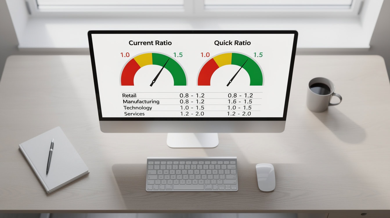
Current ratio below 1.0 is the primary liquidity distress threshold; the quick ratio below 0.5 signals an immediate cash crisis.
Profitability Ratios: Analyzing Margin Performance
Profitability ratios show how efficiently a company converts revenue into profit at three distinct levels: gross, operating, and net. All three formulas reference the Income Statement tab.
Gross Margin
What it means: The percentage of revenue remaining after subtracting the direct cost of producing goods or services (COGS). It reflects pricing power and production efficiency.
Excel formula:=IS!C5/IS!C3
Format the cell as a percentage. Excel’s percentage format multiplies the stored decimal value by 100 and displays up to 2 decimal places (Microsoft), so a formula result of 0.40 will correctly display as 40.00% without any manual adjustment.
Operating Margin
What it means: Operating income (also called EBIT, or Earnings Before Interest and Taxes) divided by revenue. EBIT is gross profit minus operating expenses like salaries, rent, and depreciation.
Excel formula:=IS!C8/IS!C3
Net Margin
What it means: Net income divided by revenue. This is the bottom-line profitability after all costs, interest, and taxes.
Excel formula:=IS!C12/IS!C3
Industry benchmarks:
| Sector | Gross Margin | Operating Margin | Net Margin |
|---|---|---|---|
| Retail | 25 – 40% | 3 – 8% | 2 – 5% |
| Manufacturing | 20 – 35% | 8 – 15% | 5 – 10% |
| Technology | 50 – 75% | 15 – 30% | 10 – 25% |
| Services | 30 – 60% | 10 – 20% | 7 – 15% |
According to data published by the U.S. Bureau of Economic Analysis, corporate profit margins across all industries averaged around 11% to 13% in recent years (Bureau of Economic Analysis).
Each margin level strips away a different cost layer: COGS for gross margin, operating expenses for operating margin, and interest plus taxes for net margin.
Worked Example: Gross Margin to Net Margin Step-by-Step
Here’s the math for a sample company with the following Income Statement figures:
- Revenue (C3): $2,000,000
- COGS (C4): $1,200,000
- Gross Profit (C5): $800,000
- Operating Income / EBIT (C8): $400,000
- Interest Expense (C10): $50,000
- Net Income (C12): $280,000
Step 1: Gross Margin=IS!C5/IS!C3 → $800,000 / $2,000,000 = 40.0%
Step 2: Operating Margin=IS!C8/IS!C3 → $400,000 / $2,000,000 = 20.0%
Step 3: Net Margin=IS!C12/IS!C3 → $280,000 / $2,000,000 = 14.0%
Interpretation: The 20-point drop from gross margin (40%) to operating margin (20%) shows that operating expenses consumed $400,000. The further drop to 14% net margin reflects $50,000 in interest and approximately $70,000 in taxes. For a services business, a 14% net margin sits comfortably above the sector median.
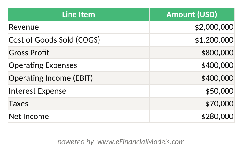
Gross Margin = Gross Profit / Revenue; Operating Margin = EBIT / Revenue; Net Margin = Net Income / Revenue. All three formulas reference the same Revenue cell.
Efficiency Ratios: Evaluating Asset and Receivables Management
Efficiency ratios (also called activity ratios) measure how productively a company uses its assets to generate revenue. These formulas mix data from both the Income Statement and Balance Sheet tabs. When using balance sheet figures in efficiency ratios, use the average of the opening and closing balance to avoid period-end distortions.
Asset Turnover
What it means: Revenue divided by average total assets. It shows how many dollars of revenue each dollar of assets generates.
Excel formula (assuming prior year total assets in column A, current year in column B):=IS!C3/((BS!A15+BS!B15)/2)
Benchmarks: Retail typically runs 1.5x to 2.5x; manufacturing 0.5x to 1.0x; technology 0.4x to 0.8x.
Receivables Turnover
What it means: Net credit sales divided by average accounts receivable. A higher number means the company collects cash from customers faster.
Excel formula:=IS!C3/((BS!A6+BS!B6)/2)
Days Sales Outstanding (DSO)
DSO converts the receivables turnover multiple into a concrete number of days. It answers: “On average, how many days does it take to collect payment after a sale?”
Excel formula:=365/(IS!C3/((BS!A6+BS!B6)/2))
Or, if you’ve already calculated receivables turnover in cell RD!B8:=365/RD!B8
Benchmarks: A DSO below 30 days is strong for most industries. Above 60 days warrants investigation into collections processes.

DSO converts the abstract receivables turnover multiple into actionable days: below 30 is strong, above 60 warrants a collections review.
Solvency Ratios: Assessing Long-Term Financial Stability
Solvency ratios measure whether a company can meet its long-term debt obligations. Unlike liquidity ratios, these look beyond the next 12 months at the overall capital structure.
Debt-to-Equity Ratio
What it means: Total debt divided by total shareholders’ equity. It shows how much of the company is financed by creditors versus owners. A ratio above 2.0 means creditors have funded more than twice what owners have contributed.
Excel formula:=BS!B18/BS!B20
Interpretation thresholds:
- Below 0.5: Conservative, low leverage.
- 0.5 to 1.5: Moderate, typical for most industries.
- Above 2.0: High leverage, red flag in capital-light sectors.
Interest Coverage Ratio
What it means: EBIT divided by interest expense. It shows how many times over a company can pay its interest bill from operating earnings. This is sometimes called the “times interest earned” ratio.
Excel formula:=IS!C8/IS!C10
Interpretation thresholds:
- Below 1.5x: Severe distress risk.
- 1.5x to 2.5x: Vulnerable; lenders will scrutinize closely.
- Above 3.0x: Comfortable coverage.
The Federal Reserve’s Senior Loan Officer Opinion Survey consistently identifies interest coverage below 2.5x as a key trigger for tightened lending standards (Federal Reserve).
Solvency benchmarks by sector:
| Sector | Debt-to-Equity | Interest Coverage |
|---|---|---|
| Retail | 0.5 – 1.5 | 3x – 8x |
| Manufacturing | 0.8 – 2.0 | 4x – 10x |
| Technology | 0.2 – 0.8 | 10x – 30x |
| Services | 0.3 – 1.0 | 5x – 15x |

Technology companies typically carry debt-to-equity below 0.8x; manufacturers may run above 1.5x due to capital-intensive operations.
Common Excel Pitfalls When Calculating Financial Ratios
Even experienced analysts make these mistakes. Here are the 5 most common errors and how to fix them.
1. Mixing statement sources
The current ratio uses only balance sheet data. Accidentally referencing a revenue cell from the income statement instead of current assets produces a meaningless number. Fix: color-code BS cells blue and IS cells green so cross-tab references are visually obvious.
2. Using period-end instead of average balance sheet figures
Efficiency ratios like asset turnover and receivables turnover should use the average of opening and closing balances, not just the year-end figure. Using only year-end data overstates or understates turnover when balances changed significantly during the year. Fix: always use =(prior_year + current_year)/2 for balance sheet inputs in efficiency formulas.
3. Circular references in linked workbooks
If your ratio dashboard references a cell that itself references the dashboard, Excel throws a circular reference error (a term for a formula that loops back to its own cell). Fix: keep raw data and calculated ratios on separate tabs with one-directional references only.
4. Hardcoding numbers instead of cell references
Typing =800000/2000000 instead of =IS!C5/IS!C3 means you must manually update every formula when data changes. Fix: always reference source cells. Use named ranges (via Formulas > Define Name) for frequently used inputs like Revenue or Total Assets. A single Excel workbook can contain up to 1,048,576 rows and 16,384 columns (Microsoft), meaning there is ample room to store multi-year historical data and named ranges without ever running out of space.
5. Forgetting to handle division-by-zero errors
If current liabilities or equity equals zero, Excel returns a #DIV/0! error. Fix: wrap formulas with IFERROR:=IFERROR(BS!B8/BS!B12, "N/A")
This keeps your dashboard clean when data is incomplete.
Using the Financial Ratio Analyzer Template
A pre-built Financial Ratio Analyzer template eliminates setup time and enforces consistent structure across every analysis. The best templates include a standardized data-entry tab for balance sheet and income statement inputs, a ratio dashboard that auto-calculates all 9 ratios the moment you enter data, conditional formatting that highlights ratios in red (distress), yellow (caution), or green (healthy) against configurable thresholds, and a trend chart section that plots each ratio across up to 5 years.
You can find ready-to-use financial analysis templates at EFM, including models that integrate ratio analysis with full three-statement models for a complete picture of financial performance. For longer planning horizons, 5-year financial projection templates include ratio tracking built into the output dashboard.
When selecting or building a template, verify that it separates input cells (unlocked, blue fill) from formula cells (locked, white fill). This prevents accidental formula overwrites. According to a study published by the European Spreadsheet Risks Interest Group, over 88% of large spreadsheets contain at least one error, with formula overwrites being among the most common causes (EuSpRIG).
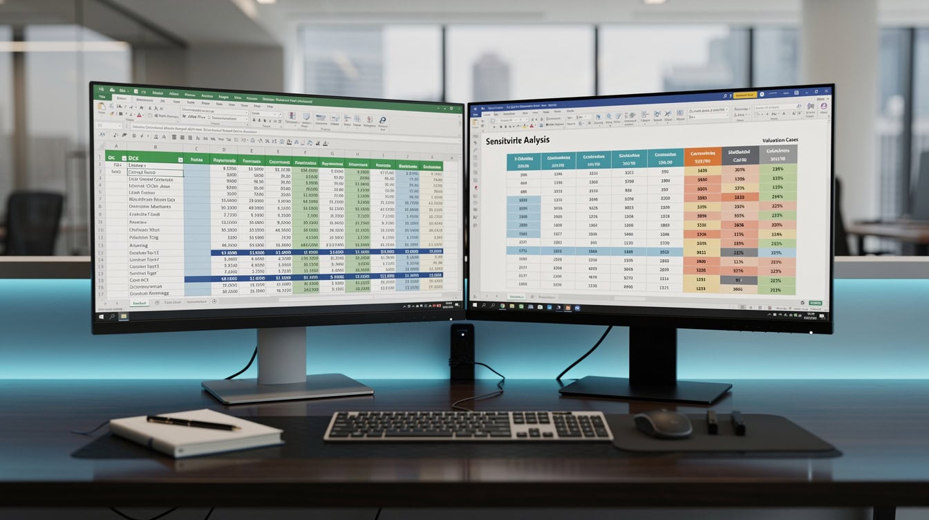
A well-designed ratio analyzer template uses conditional formatting to flag distress zones instantly, eliminating manual threshold checking.
Frequently Asked Questions
How do I calculate the current ratio in Excel with actual cell references?
The current ratio formula in Excel is =BS!B8/BS!B12, where B8 holds Total Current Assets and B12 holds Total Current Liabilities on your Balance Sheet tab. If you’re working in a single-sheet layout, the formula might be =B8/B12. Format the result as a number with 2 decimal places. A result of 1.5 means the company has $1.50 in current assets for every $1.00 of current liabilities. Anything below 1.0 is a red flag indicating the company may not cover short-term obligations without additional financing.
What is the difference between the current ratio and the quick ratio?
Both ratios measure short-term liquidity, but the quick ratio excludes inventory from current assets because inventory can take weeks or months to sell and convert to cash. The Excel formula for the quick ratio is =(BS!B8-BS!B7)/BS!B12. For a retailer with $500,000 in current assets, $200,000 in inventory, and $300,000 in current liabilities, the current ratio is 1.67 but the quick ratio drops to 1.0. That gap of 0.67 represents the liquidity risk tied up in unsold stock. Industries with slow-moving inventory, like manufacturing, show the largest spread between the two ratios.
When should I use average balance sheet figures versus period-end figures?
Use average figures whenever you pair a balance sheet item with an income statement item in the same formula. Income statement figures accumulate over the full year, so matching them against a single period-end balance sheet snapshot creates a timing mismatch. For example, asset turnover uses =IS!C3/((BS!A15+BS!B15)/2) rather than =IS!C3/BS!B15. The exception is pure balance sheet ratios like current ratio and debt-to-equity, which compare two balance sheet items from the same date and do not need averaging.
How do I prevent #DIV/0! errors in my ratio formulas?
Wrap every ratio formula in an IFERROR function. For example, instead of =BS!B8/BS!B12, write =IFERROR(BS!B8/BS!B12,"N/A"). This returns “N/A” instead of an error when the denominator is zero or blank, keeping your dashboard readable. You can also use =IF(BS!B12=0,"N/A",BS!B8/BS!B12) for more explicit control. Apply this pattern to all 9 ratio formulas from the start, especially if you’re building a template that others will populate with incomplete data.
What industry benchmarks should I use to interpret my ratios?
Benchmarks vary significantly by sector. A gross margin of 25% is healthy for retail but weak for a software company, where 70%+ is typical. For authoritative benchmarks, the U.S. Census Bureau’s Quarterly Financial Report publishes balance sheet and income statement data by industry and size class. The Federal Reserve’s Flow of Funds accounts provide aggregate corporate financial data. For public companies, you can calculate sector medians directly from SEC filings via EDGAR. Always compare your ratios against companies of similar size and business model, not just broad sector averages.
How do I build a ratio trend chart in Excel?
Calculate your ratio for each period (year or quarter) in a row across columns B through F on your Ratio Dashboard tab. Select those cells, insert a Line Chart, and label the x-axis with the period dates. For example, if your current ratio for years 2020 to 2024 sits in cells RD!B5:F5, select that range and choose Insert > Charts > Line. Add a horizontal reference line at your threshold value (e.g., 1.0 for current ratio) by adding a second data series with a constant value. This makes it immediately visible when a ratio crosses into the distress zone.
Can I calculate all 9 ratios automatically from a single data entry?
Yes. Structure your workbook so the Balance Sheet and Income Statement tabs are the only places you enter data. All 9 ratio formulas on the Ratio Dashboard tab reference those two tabs exclusively. When you update revenue or total assets, every ratio that depends on those inputs recalculates instantly. Use Excel’s data validation feature (Data > Data Validation) on input cells to restrict entries to numbers only, preventing text entries from breaking formulas. This single-entry, multi-output architecture is the core design principle behind professional financial modeling templates.
Conclusion
Calculating financial ratios in Excel becomes fast and repeatable once you separate your data inputs from your formula outputs and use consistent cell references across all 9 ratios. The 4-module structure (liquidity, profitability, efficiency, solvency) gives you a complete diagnostic view of any company’s financial health without the noise of tracking 20+ metrics simultaneously. Apply the IFERROR wrapper from day one, use average balance sheet figures for efficiency ratios, and always verify which financial statement each input comes from.
I recommend downloading the Financial Ratio Analyzer template from EFM’s financial analysis library, which includes pre-built formulas for all 9 ratios covered here, conditional formatting thresholds, and a 5-year trend dashboard, so you can start analyzing real financial statements in under 10 minutes.