0 ITEMS

CAGR Formula in Google Sheets: Copy-Paste Ready

The CAGR formula in Google Sheets takes three inputs and returns a single, comparable growth rate you can use across any business metric.
Key Takeaways
- The copy-paste CAGR formula for Google Sheets is
=POWER(B2/B1, 1/A2)-1— no add-ins or special functions required. - A SaaS company growing from $10,000 to $1,000,000 over 5 years produces a CAGR of exactly 151.19%, calculated in one cell.
- Google Sheets uses
POWER()while Excel supports bothPOWER()and theRRI()function — the syntax differs by one argument. - 3 errors account for most CAGR failures in Google Sheets:
#DIV/0!from a zero start value,#NUM!from a negative ratio, and wrong period counts from mixing years and months. - The
RATE()function offers an alternative CAGR approach for datasets with intermediate cash flows, not just start and end values. - Median SaaS revenue CAGR runs between 20% and 40% for growth-stage companies, according to OpenView Partners, giving you a benchmark to contextualize your own output.
- You can reverse the CAGR formula to find the required ending value:
=B1 * POWER(1 + target_cagr, years).
Quick Formula: Copy-Paste CAGR for Google Sheets
Paste this formula directly into any Google Sheets cell to calculate CAGR instantly:
=POWER(ending_value / starting_value, 1 / num_years) - 1With real cell references, it looks like this:
=POWER(B2/B1, 1/A2) - 1Format the result cell as a percentage (Format > Number > Percent) and you’re done. The POWER() function — which raises a number to an exponent — is available in every version of Google Sheets. Google Workspace documentation confirms no special permissions or add-ons are needed. Google Sheets supports up to 2 arguments in the POWER() function, making it straightforward to implement the CAGR exponent directly inline. Google Support provides the full function reference.
What each argument means:
ending_value / starting_value: the total growth multiple over the full period.1 / num_years: converts that total multiple into a per-year rate.- 1: strips out the original principal so you’re left with the growth rate only.

Three inputs, one formula: the POWER() function handles all the compounding math automatically.
Building Your First CAGR Calculation: Step-by-Step
Set up a three-row table in Google Sheets, enter your values, and the formula does the rest. Here’s the exact layout:
| Cell | Label | Value |
|---|---|---|
| A1 | Start Year | 2019 |
| A2 | End Year | 2024 |
| B1 | Starting Value | 50,000 |
| B2 | Ending Value | 200,000 |
| B3 | Number of Years | =A2-A1 |
| B4 | CAGR | =POWER(B2/B1, 1/B3)-1 |
Step 1: Open a new Google Sheet and type the labels in column A (rows 1 through 4).
Step 2: Enter your starting and ending values in B1 and B2.
Step 3: In B3, type =A2-A1 to calculate the number of years automatically. This prevents the most common period-counting error.
Step 4: In B4, type =POWER(B2/B1, 1/B3)-1.
Step 5: Select B4, go to Format > Number > Percent, and set decimal places to 2.
Result: $50,000 growing to $200,000 over 5 years = 31.95% CAGR.
Using $B$1 and $B$2 (absolute cell references, created by pressing F4 after selecting a cell reference) locks those cells when you copy the formula across multiple scenarios. Relative references shift automatically; absolute references stay fixed.

Using =A2-A1 for the period count (cell B3) eliminates the most common off-by-one error in CAGR calculations.
Real Example: SaaS Revenue Growth from $10K to $1M
A SaaS startup that grew monthly recurring revenue from $10,000 to $1,000,000 over exactly 5 years achieved a CAGR of 151.19%. Here’s the math:
CAGR = POWER(1,000,000 / 10,000, 1/5) - 1
     = POWER(100, 0.2) - 1
     = 2.5119 - 1
     = 1.5119
     = 151.19%
Wait — let’s be precise. $10,000 to $1,000,000 is a 100x multiple. The fifth root of 100 is 100^0.2 = 2.5119. Subtract 1 and you get 1.5119, or 151.19% CAGR.
In Google Sheets, cell B4 would show 151.19% after you enter:
=POWER(1000000/10000, 1/5)-1To put that in context: the median top-quartile SaaS company grows at roughly 50-60% annually in its early years according to OpenView Partners’ SaaS benchmarks, so 151% signals either exceptional product-market fit or a very low starting base — both worth noting in your analysis.
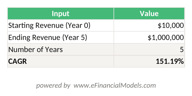
CAGR = POWER(1,000,000 / 10,000, 1/5) – 1 = 151.19%. Format cell B5 as percentage to display correctly.
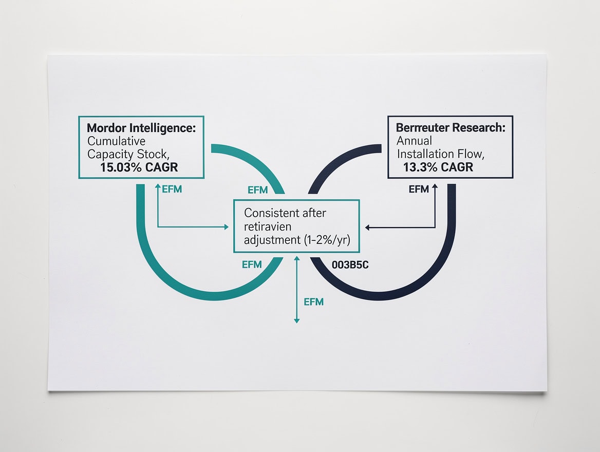
A 100x revenue multiple over 5 years produces a 151.19% CAGR — well above the 50-60% median for top-quartile SaaS companies.
Google Sheets vs Excel: CAGR Formula Differences
Both platforms can calculate CAGR, but Excel offers a dedicated RRI() function that Google Sheets does not support natively. The table below shows the exact syntax for each approach.
| Method | Google Sheets | Excel | Notes |
|---|---|---|---|
| POWER function | =POWER(end/start, 1/yrs)-1 | =POWER(end/start, 1/yrs)-1 | Identical syntax |
| Caret operator | =(end/start)^(1/yrs)-1 | =(end/start)^(1/yrs)-1 | Identical syntax |
| RRI function | Not available | =RRI(yrs, start, end) | Excel-only |
| RATE function | =RATE(yrs,0,-start,end) | =RATE(yrs,0,-start,end) | Works in both |
| XIRR function | Available | Available | Needs date array |
The RRI() function in Excel was introduced in Excel 2013 and takes exactly 3 arguments in the order (nper, pv, fv). Microsoft’s RRI function documentation provides full details. If you’re building a model that needs to run in both platforms, stick with POWER() — it’s the safest cross-platform choice.
Common CAGR Errors in Google Sheets and Fixes
Three errors cause the vast majority of broken CAGR formulas in Google Sheets. Each has a specific cause and a one-line fix.
Error 1: #DIV/0! — Starting value is zero
Cause: You divided by zero because B1 is empty or contains 0.
Fix: Wrap the formula with =IFERROR(POWER(B2/B1, 1/B3)-1, "Check start value").
Error 2: #NUM! — Negative ratio
Cause: The ending value is negative, making the ratio negative. You can’t take a fractional root of a negative number in real arithmetic.
Fix: CAGR is undefined for negative starting values. Use absolute values only if the business context supports it: =POWER(ABS(B2)/ABS(B1), 1/B3)-1. Flag the result as approximate.
Error 3: Wrong period count — mixing years and months
Cause: You entered 60 (months) in the years field instead of 5.
Fix: Always store periods in years. If your data is monthly, divide by 12 in the formula: =POWER(B2/B1, 12/num_months)-1.
Error 4: Formula returns a decimal instead of a percentage
Cause: The cell is formatted as a number, not a percentage.
Fix: Select the cell, press Ctrl+Shift+5 (Windows) or Cmd+Shift+5 (Mac) to apply percentage formatting instantly.
Error 5: CAGR looks correct but the period is off by one
Cause: Counting from 2019 to 2024 as 6 years instead of 5 (inclusive counting).
Fix: Always calculate years as End Year - Start Year, not End Year - Start Year + 1. Use =A2-A1 in a helper cell rather than hardcoding the number.

IFERROR() wrapping and explicit period calculation cells eliminate all three of the most common CAGR formula failures.
Beyond Basic CAGR: Advanced Google Sheets Techniques
Once you’ve mastered the standard formula, three advanced techniques add real analytical power to your Google Sheets CAGR work.
Reverse CAGR: Find the required ending value
If you know your starting value, target CAGR, and time horizon, solve for the required ending value:
=B1 * POWER(1 + target_cagr, years)Example: $50,000 starting value, 25% target CAGR, 4 years:
=50000 * POWER(1.25, 4) = $122,070
Quarterly data: Annualizing a quarterly CAGR
If your data points are quarterly, use the number of quarters as the period and multiply the exponent by 4:
=POWER(end/start, 4/num_quarters) - 1Multi-scenario CAGR table
Build a data table with different ending values in column B and a fixed starting value in B1. Use absolute references ($B$1) for the starting value and relative references for ending values. Copy the CAGR formula down column C to generate a full scenario range in seconds.
Alternative CAGR Functions in Google Sheets
The POWER() function isn’t the only path to CAGR in Google Sheets. Two alternatives are worth knowing.
RATE function
The RATE() function (which calculates the interest rate per period for an annuity) can compute CAGR when there are no intermediate cash flows. Google Sheets’ RATE() function accepts up to 6 arguments. Google’s RATE function documentation provides the full reference; for CAGR purposes only 4 are needed:
=RATE(num_years, 0, -starting_value, ending_value)The negative sign on starting_value is required because RATE() treats the initial investment as a cash outflow. For the $10K to $1M example over 5 years:
=RATE(5, 0, -10000, 1000000) = 151.19%This matches the POWER() result exactly. Use RATE() when you’re already working in a financial model that uses annuity functions — it keeps the formula language consistent.
XIRR function
The XIRR() function (which calculates the internal rate of return for irregular cash flows using actual dates) handles uneven time periods. If your start date is March 15, 2019 and your end date is November 3, 2024, XIRR() accounts for the partial years that POWER() would round:
=XIRR({-10000, 1000000}, {"3/15/2019", "11/3/2024"})For clean annual data, POWER() and XIRR() produce nearly identical results. For messy real-world dates, XIRR() is more accurate.

XIRR() is the most accurate option when your start and end dates don’t fall on clean annual boundaries.
When to Use CAGR vs Other Growth Metrics
CAGR smooths out volatility to show a single representative growth rate, which makes it powerful for comparisons but misleading for volatile datasets. Here’s when to use it and when to reach for something else.
| Metric | Best For | Limitation |
|---|---|---|
| CAGR | Long-term trend comparison | Hides year-to-year volatility |
| YoY Growth | Spotting annual swings | Not comparable across periods |
| MoM Growth | Early-stage SaaS tracking | Compounds to misleading annual figures |
| CAGR + Std Dev | Volatile assets | Requires more data points |
| XIRR | Irregular cash flow timing | Needs date inputs |
According to the CFA Institute curriculum, CAGR is most reliable when the underlying growth is relatively smooth and the measurement period is at least 3 years. For periods under 2 years, year-over-year percentage change is usually more informative.
CAGR Use Cases: From Startups to Enterprise Finance
CAGR applies across every stage of business and every type of metric. Five concrete scenarios show how finance professionals use it daily.
1. SaaS MRR growth tracking: A startup tracks monthly recurring revenue from $5,000 (Jan 2022) to $85,000 (Jan 2025). CAGR = POWER(85000/5000, 1/3)-1 = 189.4%. This single number goes on the investor deck.
2. Customer acquisition growth: An e-commerce brand grew its customer base from 1,200 to 18,500 over 4 years. CAGR = POWER(18500/1200, 1/4)-1 = 98.1%. Benchmark against industry peers to assess whether paid acquisition is sustainable.
3. Market share expansion: A regional insurer grew market share from 3.2% to 7.8% over 6 years. CAGR = POWER(7.8/3.2, 1/6)-1 = 15.9%. Use this to model future share targets.
4. Revenue forecasting: If last year’s revenue was $2.4M and your 3-year CAGR target is 30%, the required Year 3 revenue is =2400000 * POWER(1.3, 3) = $4.07M.
5. Portfolio benchmarking: A venture fund compares portfolio company CAGRs against the S&P 500’s historical 10-year CAGR of approximately 10.7% (according to S&P Dow Jones Indices data) to assess relative performance.
You can manage all five scenarios in a single Google Sheets financial template with named ranges and dropdown selectors.

CAGR applies to any metric with a start value, end value, and time period — from MRR to market share.
Frequently Asked Questions
What is the exact CAGR formula for Google Sheets?
The exact formula is =POWER(ending_value/starting_value, 1/num_years)-1. Replace ending_value and starting_value with your actual cell references (for example, B2 and B1), and replace num_years with the number of years in your measurement period (or a cell reference like B3). Format the result cell as a percentage. This formula works in all versions of Google Sheets without any add-ons. For example, if B1 = 100,000, B2 = 350,000, and B3 = 5, the formula returns 28.47%, meaning the investment grew at 28.47% per year on average over 5 years.
How do I calculate CAGR in Google Sheets with monthly data?
If your data points are monthly, you need to annualize the result. Use =POWER(ending_value/starting_value, 12/num_months)-1. For example, if revenue grew from $20,000 to $80,000 over 24 months, the formula is =POWER(80000/20000, 12/24)-1 = POWER(4, 0.5)-1 = 1.0 = 100%. This means revenue doubled on an annualized basis. The key is dividing 12 by the number of months rather than using the number of months directly as the exponent, which would give you a monthly rate instead of an annual one.
Why does my CAGR formula show #NUM! in Google Sheets?
The #NUM! error appears when the ratio ending_value/starting_value is negative, because Google Sheets can’t compute a real-number fractional root of a negative number. This happens when your ending value is negative (a loss position) or when you accidentally entered a negative starting value. CAGR is mathematically undefined for negative starting values. If your ending value is negative, CAGR isn’t the right metric. Use absolute dollar change or a modified Dietz return instead. If the negative sign is a data entry error, correct the source cell and the error resolves immediately.
What’s the difference between CAGR and the RATE function in Google Sheets?
Both POWER() and RATE() produce identical CAGR results for simple start-to-end growth scenarios. The syntax for RATE() is =RATE(num_years, 0, -starting_value, ending_value) — note the negative sign on the starting value, which is required because RATE() models the starting value as a cash outflow. The practical difference: RATE() is designed for annuity calculations and becomes more useful when you have periodic payments between start and end. For pure CAGR with no intermediate cash flows, POWER() is simpler and less prone to sign errors. For a $50,000 investment growing to $120,000 over 6 years, both return 15.71%.
How do I build a multi-scenario CAGR table in Google Sheets?
Create a table with different starting values in column A and different ending values in row 1. In cell B2, enter =POWER(B$1/$A2, 1/years)-1 using mixed references: B$1 locks the row (ending value stays in row 1 as you copy down) and $A2 locks the column (starting value stays in column A as you copy right). Copy this formula across the entire table. Every cell automatically calculates the CAGR for its specific starting and ending value combination. This approach is standard in financial modeling for sensitivity analysis and takes about 2 minutes to set up. You can extend it to include a fixed years input in a named cell for even more flexibility.
Can I use CAGR to forecast future revenue in Google Sheets?
Yes. The reverse CAGR formula =starting_value POWER(1 + cagr_rate, num_years) projects a future value given a known growth rate. If your current revenue is $1.5M and your target CAGR is 35%, then Year 3 projected revenue is =1500000 POWER(1.35, 3) = $3.69M. You can build a full 5-year forecast by replacing num_years with 1, 2, 3, 4, and 5 in successive cells. This is the foundation of most revenue forecasting models.
Is CAGR the same as average annual growth rate?
No, and the difference matters. CAGR (Compound Annual Growth Rate) assumes growth compounds each year, meaning each year’s growth builds on the previous year’s total. Average Annual Growth Rate (AAGR) simply averages the year-over-year percentage changes arithmetically. For a volatile dataset, AAGR will almost always be higher than CAGR. Example: an investment that grows 100% in Year 1 and falls 50% in Year 2 ends exactly where it started (net 0% gain), but AAGR = (100% + (-50%)) / 2 = 25%. CAGR correctly shows 0%. For multi-year performance comparisons, CAGR is the more accurate and widely accepted metric in financial analysis.
Conclusion
The CAGR formula in Google Sheets reduces any growth story to a single, comparable number in one cell. You’ve seen the exact formula, a worked SaaS example from $10,000 to $1,000,000, the five most common errors and their fixes, and how POWER(), RATE(), and XIRR() each serve different use cases.
I recommend downloading a financial template from EFM, which includes a pre-built CAGR calculator alongside full P&L and cash flow tracking so you can benchmark your growth rate against your actual financials in one place.