0 ITEMS

Renewable Energy Project Financial Model in Excel: Full Guide
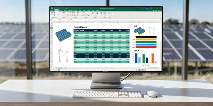
A renewable energy project financial model in Excel is the single document that determines whether your solar, wind, or battery storage deal gets funded. Get it wrong and investors walk; get it right and you close.
Key Takeaways
- Utility-scale solar capacity factors average 25-30%, onshore wind 35-45%, and offshore wind 45-55%, and these ranges drive every revenue line in your model.
- The Inflation Reduction Act sets the base Investment Tax Credit (ITC) at 30% of eligible project costs, with bonus adders that can push the effective rate to 50% or higher for qualifying projects.
- Lenders in renewable project finance typically require a minimum Debt Service Coverage Ratio (DSCR) of 1.30x-1.45x, and your model must demonstrate compliance across every year of the debt tenor.
- Solar module degradation runs approximately 0.5% per year, while wind turbine output degrades roughly 0.2% per year; failing to model these curves overstates long-term revenue by 8-12% over a 25-year project life.
- Tax equity investors in ITC flip structures typically target a 7-9% after-tax yield, and the flip point (when the investor’s ownership share drops) must be modeled precisely or your equity IRR will be wrong.
- A well-structured renewable energy Excel model separates assumptions, calculations, and outputs into distinct sheets, uses named ranges for all key inputs, and includes a scenario manager for at least 3 power price cases.
- eFinancialModels offers institutional-grade renewable energy financial model templates that include pre-built tax equity waterfalls, LCOE calculations, and technology-specific CAPEX/OPEX schedules.
What Makes Renewable Energy Financial Models Different
Renewable energy project financial models differ from conventional project finance models in four structural ways: production-based revenue (not commodity throughput), tax credit monetization through partnership structures, technology-specific degradation curves, and policy-driven economics that can shift mid-project life.
A gas plant model centers on fuel cost and spark spread. A solar or wind model centers on energy yield, which depends on irradiance or wind speed data, equipment performance, and curtailment risk. Revenue is the product of capacity factor, installed capacity, and power price, not a simple throughput margin.
The second difference is tax equity. The ITC and Production Tax Credit (PTC) are non-cash benefits that only have value if the project owner has sufficient tax appetite. Most project developers don’t. So they bring in a tax equity investor, typically a large bank or insurance company, who contributes capital in exchange for the tax credits and depreciation. This creates a partnership structure with two distinct cash flow waterfalls that must be modeled separately.
Third, renewable assets degrade. Solar modules lose approximately 0.5% of output per year according to industry performance data published by the National Renewable Energy Laboratory (NREL). Wind turbines degrade at roughly 0.2% annually. Over a 25-year project life, these curves compound into material revenue differences that a static revenue assumption will miss entirely.
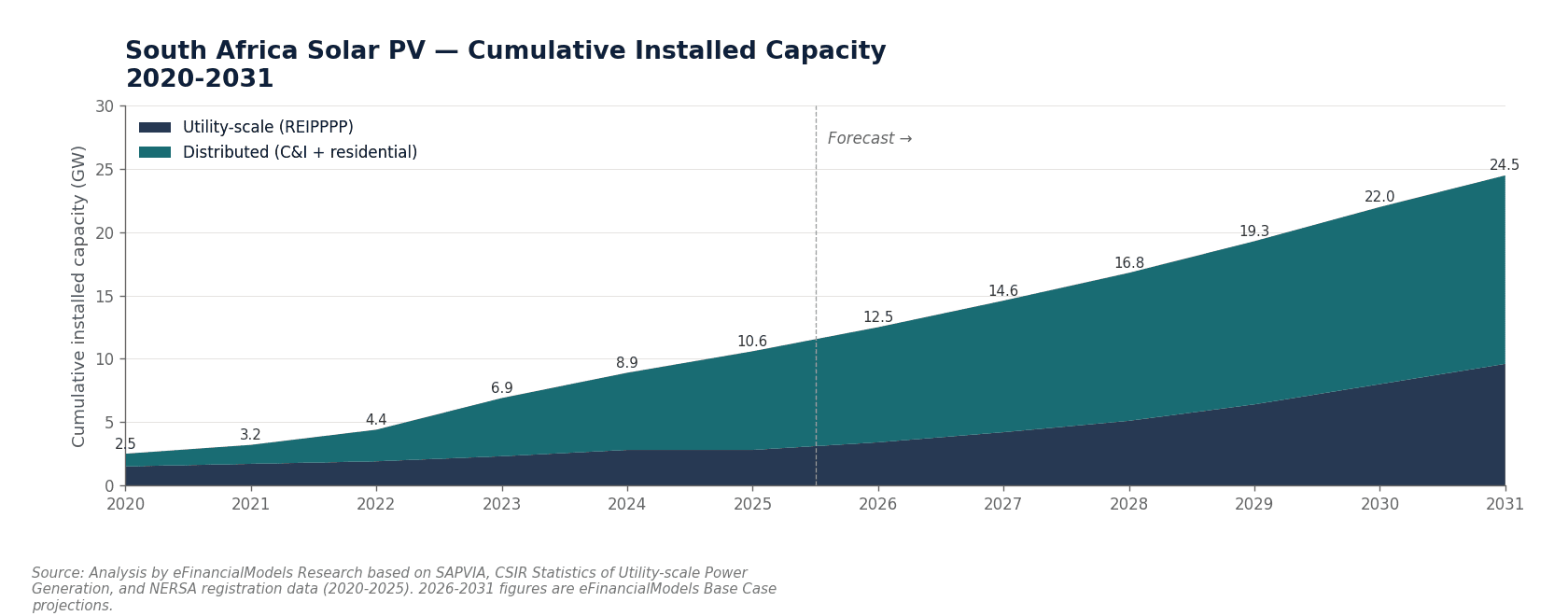
Solar degrades at 0.5%/yr, wind at 0.2%/yr, and battery storage at 2-3%/yr. Ignoring these curves overstates 25-year revenue by 8-12%.
Core Components Every Renewable Energy Excel Model Must Include
Every investor-grade renewable energy Excel model needs eight core components, each on a dedicated worksheet or clearly separated module.
1. Assumptions Dashboard. All inputs live here: installed capacity (MW), capacity factor by year, power price ($/MWh), PPA escalation rate, CAPEX per MW, O&M cost per MW-year, debt terms, tax credit type and rate, and depreciation schedule. Every other sheet pulls from this dashboard using named ranges. No hardcoded numbers anywhere else.
2. Energy Production Schedule. Annual generation (MWh) = Installed Capacity (MW) × Capacity Factor × 8,760 hours × (1 – Degradation Rate)^Year. Apply curtailment as a separate percentage reduction.
3. Revenue Model. Separate PPA revenue from merchant revenue. PPA revenue = Generation × PPA Price × (1 + Escalator)^Year. Merchant revenue uses a price curve with scenario toggles.
4. CAPEX and OPEX Schedule. CAPEX is typically front-loaded in years 0-1 (construction). OPEX includes fixed O&M ($/MW-year), variable O&M ($/MWh), land lease, insurance, and asset management fees.
5. Tax Credit and Depreciation Module. Model ITC as a percentage of eligible basis applied in year 1. Model PTC as a per-MWh credit applied over the first 10 years of operation. Apply MACRS 5-year bonus depreciation to the depreciable basis (eligible basis minus 50% of ITC for ITC projects). Excel’s NPV function (Microsoft) supports up to 254 value arguments, giving you ample room to model the full 25-year depreciation and cash flow schedule in a single formula.
6. Tax Equity Waterfall. This is the most complex component. Model the pre-flip and post-flip periods separately, allocate 99% of tax benefits to the tax equity investor pre-flip, and trigger the flip when the investor achieves its target IRR (typically 7-9%).
7. Debt Service Schedule. Model a sculpted debt service profile where annual principal payments are sized to maintain a target DSCR. Calculate DSCR = Cash Available for Debt Service (CADS) / Total Debt Service.
8. Output Dashboard. Project IRR, equity IRR, DSCR by year, LCOE, NPV at multiple discount rates, and payback period. Include a sensitivity table for power price and capacity factor.

All 8 model components pull from a single assumptions dashboard via named ranges, ensuring no hardcoded values outside the input sheet.
Building the Revenue Model: PPAs, Merchant Exposure, and Capacity Factor
Revenue in a renewable energy model flows from three sources: contracted PPA revenue, renewable energy certificate (REC) sales, and merchant or spot market exposure. Model each separately.
Power Purchase Agreements (PPAs) are long-term contracts (typically 10-20 years for utility offtakers, 7-15 years for corporate offtakers) that fix the price per MWh the project receives. The PPA price is the anchor of your revenue model. Apply an annual escalator (commonly 0-2%) and model the contract expiration explicitly, because the project’s post-PPA merchant exposure is a key risk factor for lenders.
Capacity Factor is the ratio of actual annual energy output to the theoretical maximum if the plant ran at full capacity 24/7. Use P50 (median expected output) as your base case and P90 (output exceeded 90% of the time) as your downside case. NREL’s System Advisor Model (SAM) is the industry standard tool for generating these estimates from site-specific meteorological data.
Merchant Exposure arises when the PPA expires or when a portion of output is uncontracted. Model merchant revenue using a power price forecast curve with at least three scenarios: base, low (-20%), and high (+20%). Excel’s scenario analysis tools support up to 32 changing cells per scenario (Microsoft), which is more than sufficient to toggle all key renewable energy assumptions simultaneously.
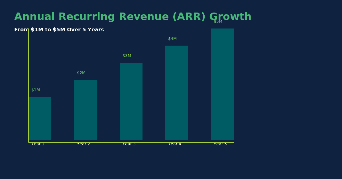
Separating PPA, REC, and merchant revenue in your model allows lenders to stress-test each stream independently.
Modeling CAPEX and OPEX for Solar, Wind, and Battery Storage
CAPEX and OPEX structures differ materially by technology, and using the wrong benchmarks will produce an unreliable model. The table below shows current industry ranges.
| Technology | CAPEX ($/W DC) | Fixed O&M ($/kW-yr) | Degradation |
|---|---|---|---|
| Utility Solar PV | $0.90-$1.10 | $15-$18 | 0.5%/yr |
| Onshore Wind | $1.20-$1.50 | $40-$50 | 0.2%/yr |
| Offshore Wind | $3.00-$4.50 | $90-$120 | 0.2%/yr |
| Battery Storage (4hr) | $250-$350/kWh | $8-$12/kWh-yr | 2-3%/yr |
For solar PV, CAPEX breaks down into modules (~25%), inverters (~8%), racking (~10%), balance of system (~20%), EPC labor (~25%), and soft costs including interconnection, permitting, and development (~12%). Model each line separately so you can stress-test individual components.
For wind, the turbine supply contract dominates CAPEX at roughly 65-70% of total project cost. Foundation and civil works, electrical collection, and substation make up the balance. O&M for wind is higher per MW than solar because of moving parts and the cost of technician access.
Battery storage CAPEX is quoted per kWh of usable energy capacity. A 100 MW / 400 MWh (4-hour) system at $300/kWh = $120M in battery CAPEX alone, before balance of system. Model battery degradation separately from solar degradation in hybrid projects.
Tax Equity Structures: ITC vs PTC Partnerships and Cash Flow Waterfalls
Tax equity is the mechanism that converts non-cash tax benefits into real project capital, and it’s the component most often modeled incorrectly. The two primary structures are the partnership flip and the sale-leaseback.
ITC Partnership Flip: The developer and tax equity investor form a partnership. The tax equity investor contributes capital (typically 35-40% of total project cost) and receives 99% of tax credits, depreciation, and cash distributions pre-flip. The flip occurs when the investor achieves its target after-tax yield (7-9%). Post-flip, the developer recaptures 95% of cash and income allocations. The developer typically holds a purchase option at fair market value.
PTC Partnership Flip: Structurally similar, but the tax benefit is the PTC (a per-MWh credit) rather than the ITC. PTC projects require the investor to remain in the partnership for the full 10-year PTC period. The Inflation Reduction Act extended and enhanced both credits: the base ITC rate is 30% of eligible project costs, and the base PTC rate is $0.0275/kWh (2024 dollars, inflation-adjusted), both subject to prevailing wage and apprenticeship requirements for the full credit amount according to the U.S. Department of Energy.
Modeling the Flip in Excel: Create a pre-flip period (years 1 through flip year) and a post-flip period. In the pre-flip period, allocate 99% of taxable income/loss and credits to the tax equity investor row. Calculate the investor’s cumulative after-tax IRR each year. When that IRR equals the target, set a flip trigger flag (1/0 binary). Use IF statements to switch allocation percentages at the flip year. Excel supports up to 64 levels of nested IF functions (Microsoft), which is far more than needed for even the most complex pre-flip and post-flip allocation logic. This is the core logic that most generic project finance models omit entirely.
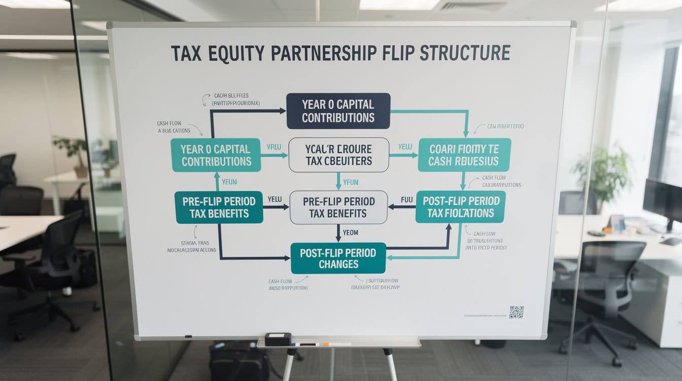
The flip trigger is a calculated output, not an input. Hardcoding the flip year is the most common tax equity modeling error.
Debt Structuring and DSCR Calculations
Renewable project finance debt is non-recourse, meaning lenders rely solely on project cash flows for repayment. This makes the DSCR the central covenant in every loan agreement.
DSCR = Cash Available for Debt Service / (Principal Repayment + Interest). Lenders in renewable project finance typically require a minimum DSCR of 1.30x-1.45x, with 1.35x being the most common covenant threshold for utility-scale solar backed by investment-grade offtakers. Projects with merchant exposure or sub-investment-grade offtakers face requirements of 1.40x-1.50x.
Debt Sculpting means sizing each year’s principal payment so that DSCR equals exactly the target ratio in every period, rather than using a flat amortization schedule. Here’s the math for a sculpted payment:
Step 1: Calculate CADS for each year = EBITDA minus taxes minus reserve funding.
Step 2: Set target DSCR = 1.35x.
Step 3: Maximum debt service = CADS / 1.35.
Step 4: Subtract interest = Maximum debt service minus interest expense.
Step 5: The result is the maximum principal repayment in that year.
This approach maximizes debt capacity (and therefore minimizes equity required) while maintaining covenant compliance. Model it using Excel’s circular reference solver or by building a debt schedule that iterates principal based on the CADS calculation.
Debt tenor typically matches the PPA length minus 1-2 years, commonly 15-18 years for a 20-year PPA. Never extend debt tenor beyond the contracted revenue period without explicit lender approval and a merchant tail analysis.
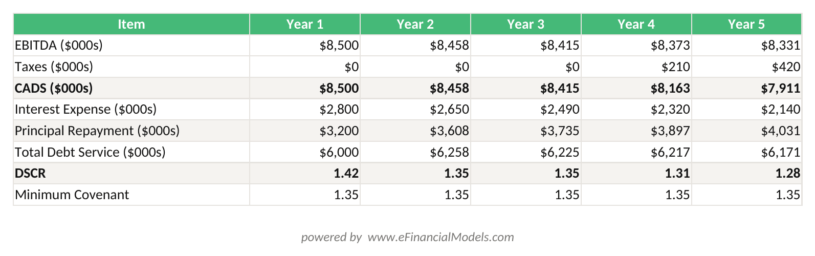
DSCR = CADS / Debt Service. Year 1 DSCR of 1.42x exceeds the 1.35x covenant minimum, confirming debt sizing is appropriate.
Key Output Metrics: IRR, NPV, LCOE, and Payback Period
Investors evaluate renewable energy projects on four primary metrics, and your model must calculate all four clearly on the output dashboard.
Project IRR is the discount rate at which the project’s NPV equals zero, calculated on pre-financing cash flows (EBITDA minus taxes minus CAPEX). A utility-scale solar project in the U.S. typically targets a project IRR of 8-12%.
Equity IRR is calculated on post-financing, post-tax equity cash flows to the developer (sponsor). This is the metric the developer cares most about. Target equity IRRs for solar sponsors typically range from 12-18% depending on risk profile and market.
LCOE (Levelized Cost of Energy) is the lifetime cost of the project divided by lifetime energy production, expressed in $/MWh. It’s the breakeven power price. LCOE = (Total Lifetime Costs, NPV) / (Total Lifetime Energy Production, NPV). Use a real discount rate (typically 5-8%) for LCOE calculations. NREL’s 2024 Annual Technology Baseline reports utility-scale solar LCOE in the range of $24-$45/MWh depending on location and financing structure.
DSCR by Year must appear as a time series, not just a single number. Lenders review the minimum DSCR across all years (the “DSCR floor”) and the average DSCR. Flag any year below the covenant threshold with conditional formatting.

The output dashboard must show DSCR as a time series, not a single number. Any year below the 1.35x covenant floor requires a structural fix.
Sensitivity Analysis and Scenario Planning
Sensitivity analysis in a renewable energy model tests how key outputs (project IRR, equity IRR, DSCR floor) respond to changes in individual input assumptions. Scenario planning tests combinations of assumptions simultaneously.
Build a two-variable data table (a native Excel feature that recalculates a formula across a grid of two input values) for project IRR as a function of power price (rows) and capacity factor (columns). Use 5 values for each variable: -20%, -10%, base, +10%, +20% relative to your base case assumption.
For scenario planning, create at least three named scenarios using Excel’s Scenario Manager or a manual toggle cell: Base Case, Downside (P90 production, low power price, 10% CAPEX overrun), and Upside (P50 production, high power price, on-budget CAPEX). Link the scenario toggle to the assumptions dashboard so all calculations update automatically.
The most impactful variables for renewable projects, ranked by typical sensitivity: (1) power price, (2) capacity factor, (3) CAPEX, (4) discount rate, (5) O&M cost escalation. Model these five in every sensitivity table.
For financial projections that need to hold up under investor scrutiny, include a Monte Carlo simulation tab or at minimum a tornado chart showing the relative impact of each variable on equity IRR.
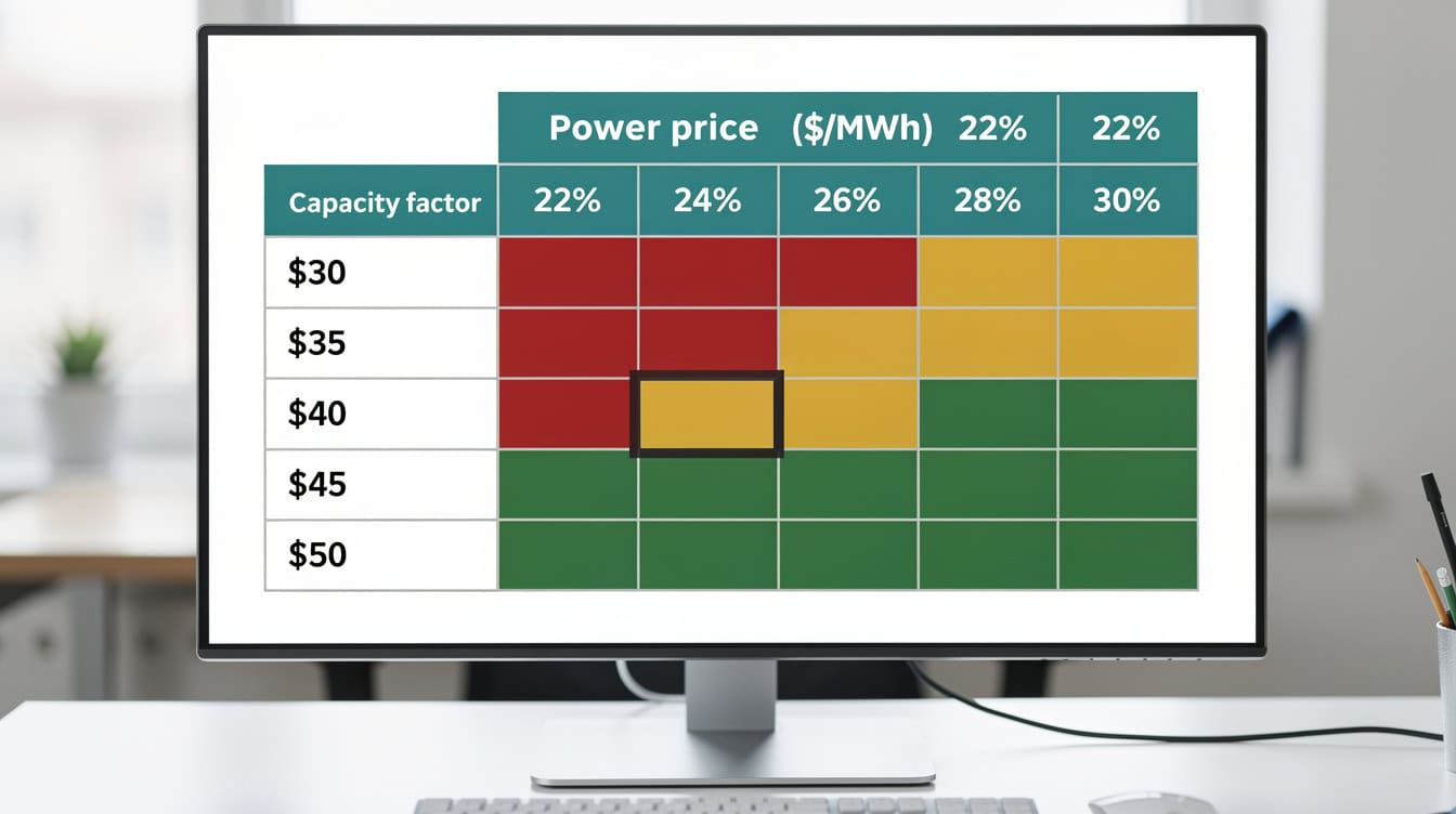
Power price is typically the most sensitive variable in a solar model, followed by capacity factor. A $5/MWh price change moves IRR by approximately 1.5-2.0 percentage points.
Common Modeling Mistakes That Kill Deals
Five specific errors appear repeatedly in renewable energy models that fail investor due diligence.
Mistake 1: Incorrect ITC Basis Calculation. The depreciable basis for MACRS depreciation must be reduced by 50% of the ITC claimed (not the full ITC). Failing to apply this “basis reduction” overstates depreciation tax shields and inflates equity IRR. Fix: In your depreciation module, set depreciable basis = eligible basis minus (0.5 × ITC amount).
Mistake 2: Misaligned Debt Tenor and PPA Length. Modeling debt that matures after the PPA expires creates a merchant tail that lenders will not accept without a significant yield premium. Fix: Set debt maturity to PPA length minus 2 years as a default, and model the merchant tail period separately with a conservative price assumption.
Mistake 3: Ignoring Curtailment. Grid curtailment (when the grid operator instructs the plant to reduce output) can reduce annual generation by 2-8% in congested markets. Fix: Add a curtailment percentage input to the assumptions dashboard and apply it as a haircut to gross generation before calculating revenue.
Mistake 4: Static Capacity Factor Across All Years. Using a single capacity factor for 25 years ignores degradation. Fix: Build a year-by-year generation schedule that applies the annual degradation rate compounded from year 1.
Mistake 5: Hardcoding Tax Equity Flip Year. Hardcoding the flip year instead of calculating it dynamically means the model breaks when you change any input that affects the investor’s IRR. Fix: Use a MATCH function to find the first year where the investor’s cumulative IRR exceeds the target, and reference that year dynamically throughout the waterfall.
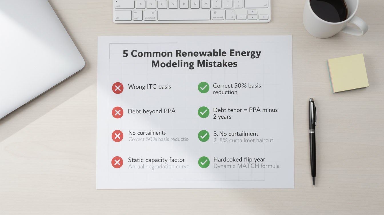
These 5 errors appear in the majority of models that fail lender due diligence. Each has a specific Excel fix that takes less than 30 minutes to implement.
Pre-Built Templates vs Custom Models: When to Use Each
For most renewable energy developers and analysts, a pre-built institutional-grade template is the right starting point. Building a full renewable energy model from scratch takes 80-120 hours for an experienced financial modeler, and the risk of structural errors in the tax equity waterfall or debt sculpting logic is high.
Pre-built templates from eFinancialModels include technology-specific configurations for solar PV, onshore wind, offshore wind, and battery storage, with pre-built ITC and PTC partnership flip structures, MACRS depreciation schedules, sculpted debt service, and a full output dashboard. These renewable energy financial model templates are designed to meet the standards of institutional lenders and tax equity investors.
Custom models make sense when: (1) your project has an unusual structure (e.g., a hybrid solar-storage-wind project with multiple offtake contracts), (2) you need to model a specific state incentive program with complex eligibility rules, or (3) your lender requires a model built to their specific template. For custom work, eFinancialModels offers custom financial modeling services tailored to project finance requirements.
The comparison below summarizes when each approach fits.
| Criterion | Pre-Built Template | Custom Model |
|---|---|---|
| Time to deploy | 1-3 days | 6-12 weeks |
| Cost | $200-$2,000 | $10,000-$50,000+ |
| Tax equity logic | Pre-built | Built to spec |
| Technology configs | Solar, wind, storage | Any |
| Lender acceptance | High (standard) | Depends on quality |
| Audit trail | Documented | Must build |
For a DCF model foundation that you can adapt for renewable projects, eFinancialModels also provides standalone discounted cash flow templates with scenario management and sensitivity tables already built in.
Frequently Asked Questions
What capacity factor should I use for a utility-scale solar project in my Excel model?
Use P50 (median expected output) as your base case and P90 as your downside. For utility-scale solar in the U.S., P50 capacity factors typically range from 25% to 30% depending on location, with the Southwest (Arizona, Nevada, New Mexico) at the high end and the Northeast at the low end. NREL’s PVWatts calculator and System Advisor Model (SAM) generate site-specific P50 and P90 estimates from 30 years of meteorological data. Always source your capacity factor from a third-party energy assessment report for any project seeking project finance debt, because lenders will require it. Using a generic 27% without a site-specific study is a common reason models fail due diligence at the lender review stage.
How do I model the ITC in Excel for a solar project?
The ITC (Investment Tax Credit) under Section 48 of the Internal Revenue Code equals 30% of the eligible project basis for projects meeting prevailing wage and apprenticeship requirements, according to the U.S. Department of Energy. In your Excel model, calculate eligible basis as total CAPEX minus land costs minus certain interconnection costs. Apply the ITC in year 1 of operations as a tax credit (a direct reduction in tax liability, not a deduction). Then reduce the depreciable basis by 50% of the ITC amount before calculating MACRS depreciation. For a $100M eligible basis: ITC = $30M, depreciable basis = $100M minus $15M = $85M. Apply 5-year MACRS to $85M. This two-step calculation is where most models introduce errors.
What DSCR do renewable energy lenders require?
Renewable project finance lenders typically require a minimum DSCR of 1.30x to 1.45x, with the specific covenant depending on offtake quality, technology, and market. A utility-scale solar project with a 20-year PPA from an investment-grade utility will typically achieve a 1.35x minimum DSCR covenant. Projects with merchant exposure, shorter PPAs, or sub-investment-grade offtakers face requirements of 1.40x to 1.50x. Your model must show the DSCR in every year of the debt tenor, flag any year below the covenant with conditional formatting, and calculate both the minimum DSCR (the floor lenders focus on) and the average DSCR across the full debt period. A single year below 1.30x will typically require a reserve account or structural fix before lenders will proceed.
What is LCOE and how do I calculate it in Excel?
LCOE (Levelized Cost of Energy) is the minimum power price at which a project breaks even on a net present value basis over its full operating life. It’s expressed in $/MWh and is the standard metric for comparing the economics of different generation technologies. The formula is: LCOE = NPV of all lifetime costs / NPV of all lifetime energy production. In Excel, calculate the NPV of costs using the NPV function with a real discount rate (typically 5-8%) applied to the annual cost stream (CAPEX in year 0, O&M in years 1-25). Calculate the NPV of energy production using the same discount rate applied to the annual MWh output stream. Divide the two NPVs. NREL’s 2024 Annual Technology Baseline reports utility-scale solar LCOE in the range of $24-$45/MWh, which is a useful sanity check for your model output.
How long does a PPA typically last for a renewable energy project?
PPA contract lengths vary by offtaker type. Utility offtakers (investor-owned utilities, municipal utilities, cooperatives) typically sign 15-25 year PPAs, with 20 years being the most common for utility-scale solar and wind. Corporate offtakers (tech companies, manufacturers) typically sign 10-15 year PPAs. Shorter corporate PPAs create a merchant tail that must be modeled explicitly, because lenders will not extend debt beyond the contracted revenue period without a significant risk premium. In your Excel model, build a PPA expiration flag that switches revenue from contracted PPA pricing to a merchant price curve at the contract end date. The post-PPA merchant period is often the most sensitive part of the model for equity IRR.
What is a tax equity flip structure and why does it matter for my model?
A tax equity flip structure is a partnership arrangement where a tax equity investor (typically a large bank or insurance company) contributes capital to a renewable energy project in exchange for the majority of tax credits and depreciation benefits. The flip is the point at which the investor’s ownership share drops from 99% to 5% after the investor achieves its target after-tax yield, typically 7-9%. This structure matters for your model because it creates two distinct cash flow periods with different allocation percentages, and the flip year is a calculated output (not an input) that depends on the investor’s cumulative IRR. If you hardcode the flip year or use a simplified single-waterfall structure, your equity IRR calculation will be wrong. The developer’s cash flows are minimal pre-flip and substantial post-flip, so the flip timing directly determines the developer’s equity IRR.
Can I use a pre-built Excel template for a real investor pitch?
Yes, provided the template meets institutional standards. An investor-grade renewable energy Excel model must include: a locked assumptions dashboard with all inputs in one place, dynamic tax equity waterfall with calculated flip year, sculpted debt service with DSCR by year, technology-specific degradation curves, sensitivity tables for power price and capacity factor, and a clean output dashboard with project IRR, equity IRR, LCOE, and NPV. eFinancialModels’ renewable energy financial model templates are built to these standards and have been used in transactions reviewed by institutional lenders and tax equity investors. For a first investor meeting or lender term sheet process, a well-configured pre-built template is entirely appropriate. For financial close, you may need to adapt the model to the lender’s specific requirements.
Conclusion
A renewable energy project financial model in Excel is not a generic DCF with a green label. It requires technology-specific production curves, a dynamic tax equity waterfall, sculpted debt service, and output metrics that institutional investors and lenders can audit and trust. The five modeling mistakes covered above (incorrect ITC basis, misaligned debt tenor, ignored curtailment, static capacity factor, hardcoded flip year) are the most common reasons deals stall in due diligence.
I recommend downloading eFinancialModels’ institutional-grade renewable energy financial model templates as your starting point. These templates include pre-built ITC and PTC partnership flip structures, MACRS depreciation, sculpted debt service, and a full sensitivity dashboard, saving you 80-120 hours of build time and reducing the risk of structural errors that kill deals.