0 ITEMS

Balance Sheet in Excel: Formulas, Tips & Templates
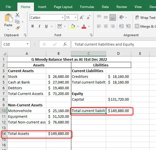
Excel is still the fastest way to build a balance sheet that actually balances — as long as the formulas, formatting, and error checks are set up correctly from the start. Here is a quick summary of what matters most, followed by a full walkthrough and templates you can reuse.
Key Takeaways
- The accounting equation Assets = Liabilities + Equity must balance to zero; use
=SUM(B4:B15)-SUM(D4:D12)-SUM(F4:F8)as a live check cell that flags any discrepancy instantly. - Excel worksheets support up to 1,048,576 rows and 16,384 columns, giving enterprise finance teams room to track thousands of line items without splitting workbooks.
- Separate input cells (yellow fill) from formula cells (locked, grey fill) to prevent accidental overwrites that corrupt your balance sheet totals.
- Named ranges such as
TotalAssetsandTotalLiabilitiesmake formulas readable and reduce broken-reference errors when rows are inserted or deleted. - A workbook can hold up to 1,024 unique cell formats, so reuse a defined set of 6 to 8 cell styles rather than applying ad-hoc formatting that exhausts the limit.
- Conditional formatting rules that turn negative equity red and flag an unbalanced sheet in orange give reviewers an instant visual audit without opening a single formula.
- Microsoft 365 Copilot can generate balance sheet formulas and summarize period-over-period changes in plain English, cutting first-draft build time significantly for users on eligible plans.
Excel has been the default financial reporting tool since Microsoft Office first shipped in 1989 (Encyclopaedia Britannica). Decades later, it still powers balance sheets at firms ranging from solo consultants to Fortune 500 finance teams. The difference between a fragile spreadsheet and a professional-grade balance sheet comes down to three things: formula architecture, formatting discipline, and error prevention. This guide covers all three with exact syntax and real numbers.
Understanding Balance Sheet Structure in Excel
A balance sheet reports a company’s financial position at a single point in time using three sections: assets (what the company owns), liabilities (what it owes), and equity (the residual interest of the owners). The fundamental accounting equation is Assets = Liabilities + Equity, and every formula decision in your Excel model flows from that constraint.
Current assets are resources expected to convert to cash within 12 months: cash, accounts receivable, and inventory. Non-current assets include property, plant and equipment (PP&E) and intangible assets. On the other side, current liabilities cover obligations due within 12 months (accounts payable, short-term debt), while non-current liabilities include long-term loans and deferred tax. Equity holds paid-in capital and retained earnings.
Public companies in the United States must file balance sheets as part of their annual Form 10-K and quarterly Form 10-Q reports with the U.S. Securities and Exchange Commission (SEC). Many large filers also tag their balance sheet data using the XBRL U.S. taxonomy, a standardized machine-readable format that regulators and analysts use to compare statements across companies (XBRL US). Even if you never file with the SEC, structuring your Excel balance sheet to mirror these conventions makes it easier to hand off to auditors or lenders.
Setting Up Your Excel Balance Sheet Template
A well-structured template separates three types of cells: input cells where users type raw data, calculation cells that contain formulas, and label cells that hold text only. This separation is the single most important design decision you will make.
Recommended layout (columns A through F):
- Column A: Line item labels (e.g., “Cash and Cash Equivalents”)
- Column B: Current period values
- Column C: Prior period values
- Column D: Change (formula:
=B4-C4) - Column E: % Change (formula:
=IFERROR(D4/C4,"N/A"))
Step-by-step template setup:
- Open a new workbook. Rename Sheet1 to “Balance Sheet” and Sheet2 to “Inputs”.
- On the Inputs sheet, list all raw data entries (cash balance, receivables, etc.) with yellow-filled cells. Use Data Validation (Data tab > Data Validation) to restrict numeric cells to numbers only.
- On the Balance Sheet sheet, reference Inputs cells using
=Inputs!B2style links. Never type a number directly into a formula cell. - Create named ranges: select B4:B15 (your current asset values), go to Formulas > Define Name, and enter
CurrentAssets. Repeat for liabilities and equity ranges. - Add a “Check” cell at the top:
=TotalAssets-TotalLiabilities-TotalEquity. Format it with conditional formatting: green fill if the result equals zero, red fill if it does not. - Protect the Balance Sheet sheet (Review > Protect Sheet) with a password, leaving only the Inputs sheet editable.
A single Excel workbook can contain up to 255 sheets (Microsoft Support), so you have ample room to keep your Inputs, Balance Sheet, and historical period tabs all within one file without splitting across workbooks.
Essential Excel Formulas for Balance Sheet Automation
The right formulas eliminate manual recalculation and catch errors before they reach a reviewer. Here are the core functions every balance sheet builder needs.
SUM for section totals:
=SUM(B4:B15)   ' Total current assets
=SUM(B18:B22)  ' Total non-current assets
=B16+B23       ' Grand total assets
SUMIF for category aggregation (useful when your data lives in a flat transaction list on another sheet):
=SUMIF(Inputs!A:A,"Current Asset",Inputs!B:B)SUMIF (a conditional sum function) scans column A of the Inputs sheet for the text “Current Asset” and adds the corresponding values in column B.
INDEX-MATCH for pulling prior-period comparatives from a historical data table:
=INDEX(HistoricalData!B:B, MATCH(A4, HistoricalData!A:A, 0))INDEX-MATCH (a lookup combination that returns a value from a specified position) is more robust than VLOOKUP because it works with columns in any order and does not break when you insert columns.
IFERROR for clean error handling:
=IFERROR(D4/C4, "N/A")This prevents #DIV/0! errors in the % Change column when a prior-period value is zero.
The balance check formula (the most important formula in the entire model):
=IF(ABS(TotalAssets-(TotalLiabilities+TotalEquity))<0.01,"BALANCED","ERROR: "&TEXT(ABS(TotalAssets-(TotalLiabilities+TotalEquity)),"$#,##0.00")&" OUT OF BALANCE")The ABS function (absolute value, stripping any negative sign) and a 0.01 tolerance handle rounding differences from currency conversions.
Excel formulas can contain up to 8,192 characters (Microsoft Support), so even the most complex nested balance check will fit within a single cell.
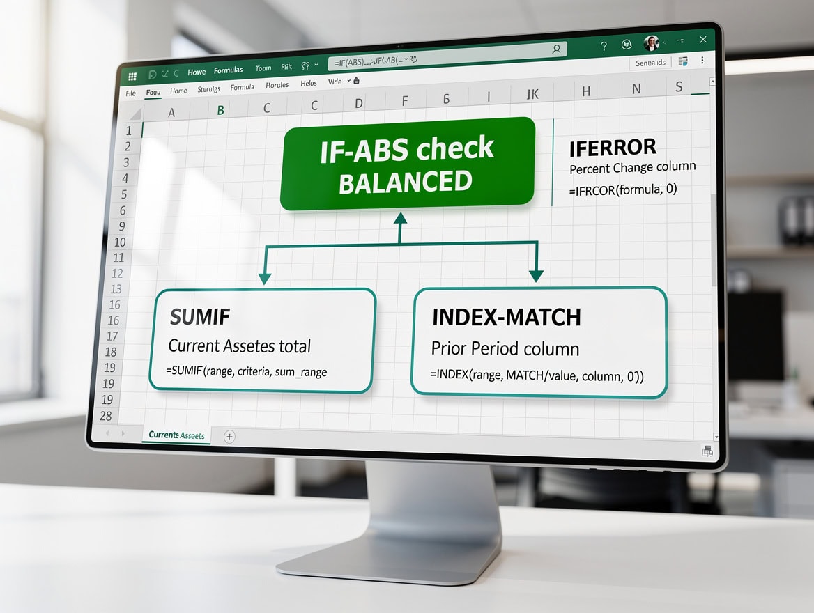
Four formula types handle 90% of balance sheet automation: SUMIF for aggregation, INDEX-MATCH for lookups, IFERROR for clean errors, and IF-ABS for the balance check.
Worked Numerical Example: Building the Balancing Check
Here’s the math for a simplified balance sheet with three asset lines, two liability lines, and one equity line.
Inputs (on the Inputs sheet):
- B2: Cash = $50,000
- B3: Accounts Receivable = $30,000
- B4: Inventory = $20,000
- B6: Accounts Payable = $25,000
- B7: Long-Term Debt = $40,000
- B9: Retained Earnings = $35,000
Balance Sheet sheet formulas:
- Total Assets cell (B16):
=SUM(B4:B6)= $50,000 + $30,000 + $20,000 = $100,000 - Total Liabilities cell (D10):
=SUM(D4:D5)= $25,000 + $40,000 = $65,000 - Total Equity cell (F6):
=F4= $35,000 - Check cell (B2):
=B16-(D10+F6)= $100,000 – ($65,000 + $35,000) = $0 (BALANCED)
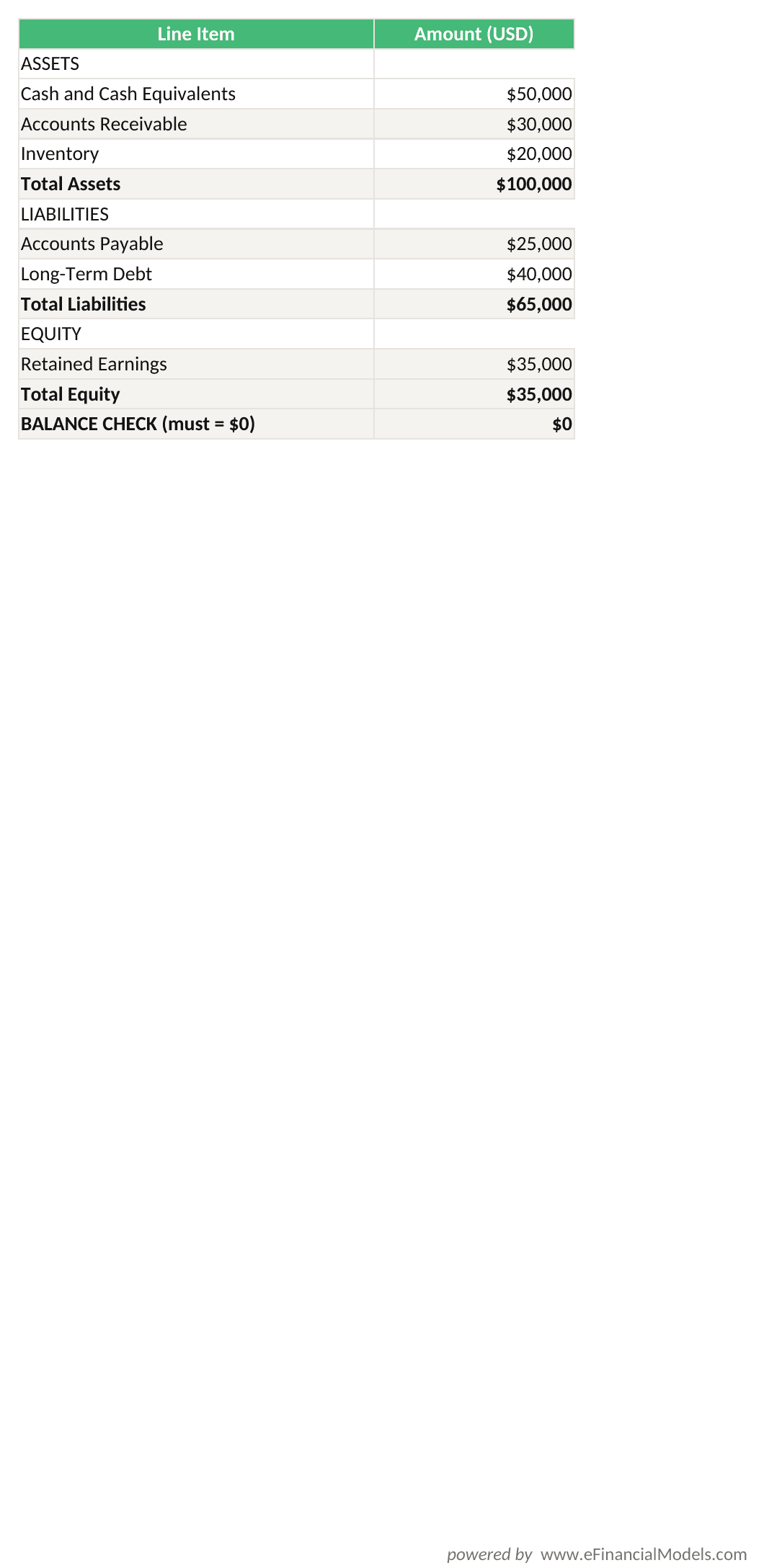
Balance Check = TotalAssets – (TotalLiabilities + TotalEquity). Result must equal $0 for the sheet to be in balance.
If the check cell returns anything other than zero, the model is out of balance. The most common cause is a line item entered on the wrong side of the equation, which the check cell surfaces immediately.
Professional Formatting and Presentation Techniques
Formatting is not cosmetic. A poorly formatted balance sheet causes reviewers to misread figures, miss sign conventions, and lose trust in the numbers. Apply these rules consistently.
Currency formatting: Select all value cells, press Ctrl+1 to open Format Cells, choose Number > Accounting, set decimal places to 0 for round-number reports or 2 for detailed statements. The Accounting format aligns currency symbols and decimal points in a column, making vertical comparisons easy.
Conditional formatting rules to set up:
- Negative equity: Select the equity section, apply a rule “Cell Value < 0”, set fill to red and font to white.
- Unbalanced sheet: Select the check cell, apply “Cell Value <> 0”, set fill to orange.
- Large year-over-year swings: Select the % Change column, apply a 3-color scale (green for positive, yellow for neutral, red for negative).
A single worksheet supports up to 64,000 conditional formatting rules (Microsoft Support), so even a highly annotated balance sheet with rules on every section will not approach that ceiling.
Cell styles for consistency: A workbook supports up to 1,024 unique cell formats (Microsoft Support), so define a small palette of named styles (Header, SubHeader, InputCell, FormulaCell, TotalRow) and apply them from the Home > Cell Styles gallery. This keeps your format count low and your sheet visually consistent.
Borders and shading: Use thick bottom borders on subtotal rows and double bottom borders on grand total rows. This mirrors the convention in audited financial statements and signals to readers where to look for key figures.

Conditional formatting rules surface balance errors and negative equity instantly, without requiring a reviewer to inspect individual formulas.
Data Validation and Error Prevention Strategies
Error prevention is cheaper than error correction. Build these checks into the template before anyone enters data.
Data validation on input cells:
- Restrict numeric cells to whole numbers or decimals only (Data > Data Validation > Allow: Decimal).
- Add an input message: “Enter value in USD, no commas” to guide users.
- Set an error alert to “Stop” so Excel rejects non-numeric entries outright.
Circular reference detection: A circular reference occurs when a formula refers back to its own cell, either directly or through a chain of other cells. Excel flags these with a status bar warning. To find them, go to Formulas > Error Checking > Circular References. Balance sheets rarely need circular references; if you see one, it usually means a retained earnings formula is incorrectly referencing the net income cell on the same sheet.
Named range audit: Go to Formulas > Name Manager to review all named ranges. Delete any that point to #REF! errors, which happen when the rows a named range referenced have been deleted.
Worksheet protection: After building the template, protect all formula cells (select them, Ctrl+1 > Protection > Locked = checked) and then protect the sheet (Review > Protect Sheet). Leave only input cells unlocked. This prevents the most common source of balance sheet errors: someone overwriting a SUM formula with a hardcoded number.

Data validation, named ranges, and sheet protection form a three-layer error prevention system for professional balance sheet templates.
Using PivotTables for Multi-Period Balance Sheet Analysis
PivotTables (Excel’s dynamic summarization tool that reorganizes and aggregates data without altering the source) let you compare balance sheet snapshots across multiple periods without building separate sheets for each quarter.
Setup steps:
- Structure your historical data as a flat table with columns: Date, LineItem, Category, Amount.
- Select the table and insert a PivotTable (Insert > PivotTable).
- Drag Date to Columns, LineItem to Rows, and Amount to Values (set to Sum).
- Group the Date field by Quarter or Year (right-click a date cell > Group).
- Add a slicer for Category (Insert > Slicer) so you can filter to Assets, Liabilities, or Equity with one click.
This setup turns a multi-year dataset into a comparative balance sheet in under five minutes. When new period data arrives, right-click the PivotTable and select Refresh to update all figures instantly.
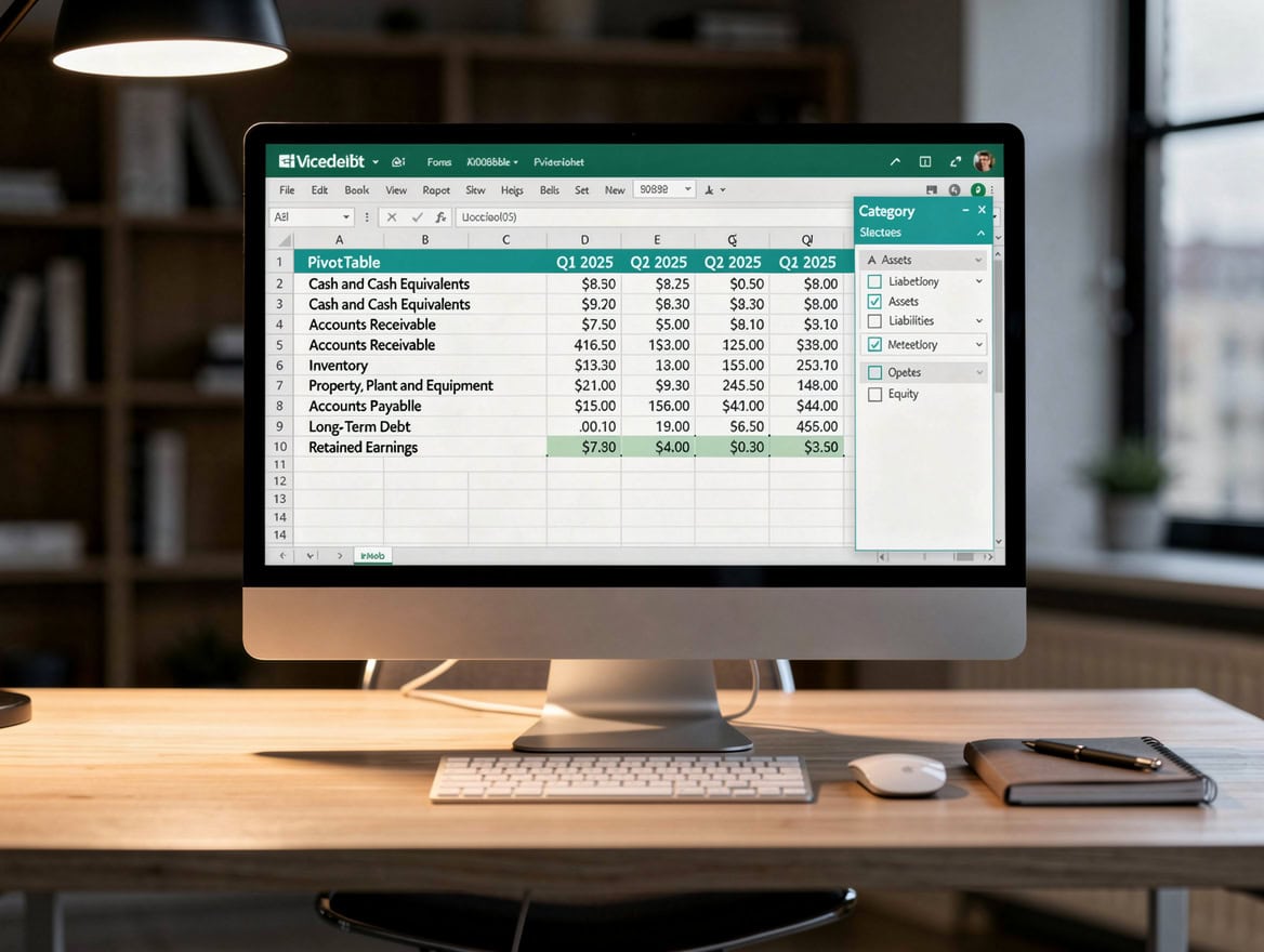
A PivotTable built from a flat data table turns multi-year balance sheet data into a comparative view that refreshes in one click.
Microsoft 365 Copilot for Balance Sheet Creation
Microsoft 365 Copilot can analyze data in Excel and generate formulas, charts, and summaries directly from your spreadsheet (Microsoft Support). For balance sheet work, Copilot is most useful in three scenarios.
First, formula generation: type a plain-English prompt such as “Write a formula that sums all rows in column B where column A contains ‘Current Asset'” and Copilot returns the correct SUMIF syntax. This is faster than looking up syntax for analysts who use SUMIF infrequently.
Second, anomaly detection: ask Copilot to “Highlight any line items where the year-over-year change exceeds 50%” and it applies conditional formatting automatically.
Third, narrative summaries: Copilot can draft a plain-English paragraph describing the period-over-period changes in your balance sheet, useful for board packs or management commentary sections.
Copilot requires a Microsoft 365 Business Standard or higher subscription. It does not replace formula knowledge, but it accelerates first-draft work and reduces syntax lookup time.
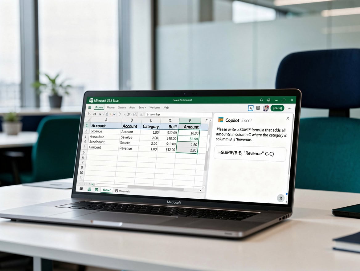
Copilot accelerates formula generation and anomaly detection but requires a Microsoft 365 Business Standard or higher subscription.
Common Excel Balance Sheet Mistakes and How to Fix Them
Five mistakes account for the majority of balance sheet errors in Excel. Here’s each one with a specific fix.
| Mistake | What Goes Wrong | Fix |
|---|---|---|
| Hardcoded values in formula cells | Someone types 100000 instead of referencing the Inputs sheet; future updates miss that cell | Lock formula cells with sheet protection; use Find & Replace (Ctrl+H) to audit for hardcoded numbers |
| Missing sign convention | Liabilities entered as positive when the check formula expects them as negative (or vice versa) | Standardize: all values positive, and let the check formula subtract liabilities from assets |
| Broken named ranges after row insertion | Inserting a row above a named range shifts the reference, causing #REF! errors | Use table-structured references (Excel Tables auto-expand) or audit Name Manager after any structural change |
| Unprotected formula cells | A user overwrites =SUM(B4:B15) with a static number; the sheet still looks balanced but is wrong | Protect the sheet before distributing; use Formulas > Show Formulas (Ctrl+`) to audit periodically |
| No balance check cell | Errors accumulate silently across multiple periods | Add the IF/ABS check formula described above to every version of the template |
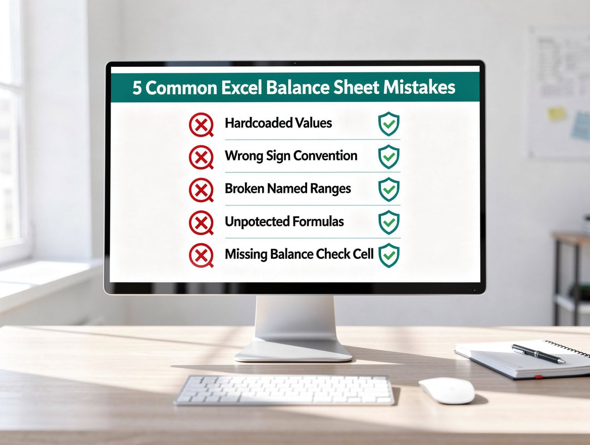
These five mistakes account for the majority of balance sheet errors in Excel; each has a specific, preventable fix.
Frequently Asked Questions
What is the exact Excel formula to verify a balance sheet balances?
The most reliable check formula is =IF(ABS(TotalAssets-(TotalLiabilities+TotalEquity))<0.01,"BALANCED","OUT OF BALANCE BY "&TEXT(ABS(TotalAssets-(TotalLiabilities+TotalEquity)),"$#,##0.00")). Place this in a prominently colored cell at the top of your balance sheet. The 0.01 tolerance handles rounding differences that arise when values are sourced from systems that round to the nearest cent differently. If the cell displays anything other than “BALANCED”, trace the discrepancy by checking each section total against its source data on the Inputs sheet. Named ranges like TotalAssets make this formula readable and maintainable across template versions.
How do I use SUMIF to categorize balance sheet line items automatically?
SUMIF is a conditional sum function that adds values in a range only when a corresponding cell meets a criterion. For a balance sheet, set up a flat data table on a separate sheet with columns for LineItem, Category (e.g., “Current Asset”, “Non-Current Asset”), and Amount. Then on your balance sheet, use =SUMIF(Data!B:B,"Current Asset",Data!C:C) to pull the total for that category. This approach means you only enter data once and the balance sheet sections populate automatically. It also makes adding new line items trivial: add a row to the data table with the correct category label and the balance sheet updates on the next calculation cycle.
What is the best way to handle negative values on a balance sheet in Excel?
The cleanest convention is to enter all values as positive numbers and let the accounting equation handle the sign logic in your check formula. Avoid entering liabilities as negative numbers unless your model explicitly requires it, because mixed sign conventions are the leading cause of balance sheet errors in Excel. Apply conditional formatting to flag any cell in the equity section that goes negative (a red fill rule on “Cell Value < 0”) so that negative equity, which can be a legitimate but significant condition, is immediately visible to reviewers. For presentation, use the Accounting number format, which displays negative values in parentheses rather than with a minus sign, matching audited financial statement conventions.
How do I create a comparative balance sheet for multiple periods in Excel?
The most scalable approach uses a flat data table with a Date column and a PivotTable to display periods side by side. Structure your source data as: Date | LineItem | Category | Amount. Insert a PivotTable with LineItem in Rows, Date in Columns (grouped by quarter or year), and Amount in Values. This gives you a comparative balance sheet that updates with one click when new period data is added. For a simpler two-period comparison, add a Prior Period column to your standard template and use =INDEX(HistoricalData!B:B,MATCH(A4,HistoricalData!A:A,0)) to pull prior figures. Always include a % Change column using =IFERROR((B4-C4)/C4,"N/A") to surface material movements.
How do I protect formulas in an Excel balance sheet without locking the whole sheet?
Excel’s protection model works at the cell level first, then the sheet level. By default, all cells are marked as “Locked” in Format Cells > Protection, but locking only activates when you protect the sheet. The workflow is: (1) Select all cells with Ctrl+A, open Format Cells (Ctrl+1), go to Protection, and uncheck Locked. (2) Select only your formula cells, open Format Cells again, and check Locked. (3) Go to Review > Protect Sheet, set a password, and check “Select unlocked cells” so users can still navigate to input cells. This lets users type in yellow input cells freely while preventing any edits to formula cells. Distribute the password only to template maintainers.
Can Excel handle enterprise-scale balance sheets with thousands of line items?
Yes. Excel worksheets support up to 1,048,576 rows and 16,384 columns (Microsoft Support), which is more than sufficient for even the most detailed enterprise chart of accounts. Performance becomes the practical constraint before capacity does. For large models, convert your data ranges to Excel Tables (Ctrl+T) so formulas use structured references that recalculate only affected cells. Avoid volatile functions like INDIRECT and OFFSET in large balance sheets because they recalculate every time any cell in the workbook changes, which slows down large files noticeably.
What is XBRL and does it affect how I structure my Excel balance sheet?
XBRL (eXtensible Business Reporting Language) is a standardized tagging system that makes financial statement data machine-readable. The XBRL U.S. taxonomy defines specific element names for every balance sheet line item, such as “us-gaap:CashAndCashEquivalentsAtCarryingValue” for cash (XBRL US). If your company files with the SEC, your finance team or auditors will map your Excel line items to XBRL tags during the filing process. You can make that mapping easier by labeling your Excel line items consistently with standard accounting terminology (“Cash and Cash Equivalents” rather than “Cash on Hand”) and keeping one row per line item rather than combining items. This alignment also makes your balance sheet easier to compare against peers and industry benchmarks.
Build Your Balance Sheet Right the First Time
A professional Excel balance sheet is not just a formatted table. It is a system: structured inputs, formula-driven calculations, automated error checks, and protected cells that prevent silent corruption. The accounting equation Assets = Liabilities + Equity is simple, but enforcing it reliably across dozens of line items and multiple periods requires deliberate template design.
Start with the balance check formula. Add named ranges before you write a single SUM. Protect formula cells before you share the file. These three steps alone eliminate the majority of balance sheet errors that finance teams spend hours debugging.
For Excel financial models that go beyond the balance sheet, including integrated income statements and cash flow statements, the structure principles are identical: separate inputs from calculations, name your ranges, and build a check. The General Excel Financial Models library at EFM contains templates that apply all of these conventions out of the box.
I recommend downloading the EFM professional Excel balance sheet template to get a pre-built, formula-driven starting point with named ranges, conditional formatting, and a live balance check cell already configured. It will save you two to three hours of setup time and give you a structure you can adapt for any reporting period or industry.