0 ITEMS

Amortization Schedule in Excel: Build One in 9 Steps
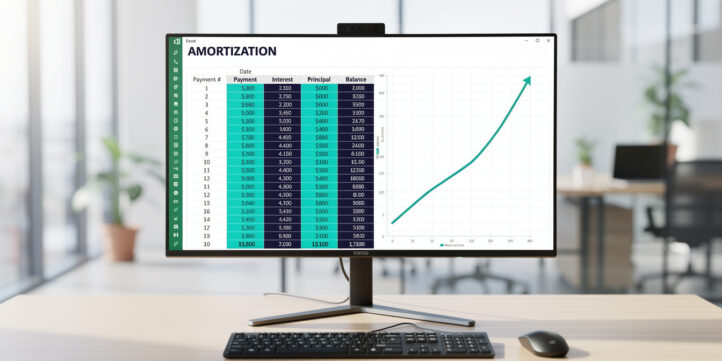
A loan amortization schedule breaks every payment into its interest and principal components, period by period, so you can see exactly how a debt unwinds over time. This guide walks you through building one from scratch in Excel using the PMT, IPMT, and PPMT functions, with real numbers, validation checks, and professional formatting.
Key Takeaways
- Excel’s PMT function calculates a fixed periodic payment in one formula:
=PMT(rate/periods, nper, -pv), where dividing the annual rate by payment frequency is the single most common mistake practitioners make. - A 30-year, $300,000 mortgage at 6.5% annual interest generates 360 rows of data; using absolute cell references (the
$sign) for your input parameters is what makes the entire schedule dynamic. - The first payment on that mortgage allocates roughly $1,625 to interest and only $275 to principal, illustrating why early payoff saves disproportionately more money.
- Excel’s IPMT and PPMT functions let you calculate interest and principal for any single period without building the full schedule, which is useful for spot-checking your row formulas.
- Rounding errors compound across 360 periods; the final payment in a correctly built schedule will differ from all others by a few cents, and you should handle this with an IF formula rather than ignoring it.
- Extra payment functionality, balloon payments, and variable rate toggles can all be added with conditional logic, turning a static schedule into a full loan analysis tool.
- A sum-check row that verifies total interest paid against the theoretical figure is the fastest way to confirm your schedule is error-free before sending it to a client.
Understanding Amortization: The Financial Mechanics Behind Loan Repayment
Amortization is the process of paying off a debt through scheduled, equal payments where each installment covers accruing interest first, with the remainder reducing the outstanding principal. The word comes from the Old French amortir, meaning to kill off, which is exactly what happens to the loan balance over time.
The mathematical foundation is the present value of an annuity formula. For a fixed-rate loan, the periodic payment (PMT) is:
PMT = PV × r(1+r)^n / (1+r)^n – 1
Where:
- PV = present value (loan principal)
- r = periodic interest rate (annual rate divided by number of payments per year)
- n = total number of payment periods
This formula ensures that the sum of all discounted future payments equals the loan principal today. The Federal Reserve’s consumer credit guidelines confirm that this constant-payment, declining-balance structure is the standard for virtually all consumer and commercial installment loans in the United States.
The interest portion of each payment equals the outstanding balance multiplied by the periodic rate. Because the balance falls with every payment, the interest component shrinks and the principal component grows, even though the total payment stays constant. This is the defining characteristic of a fully amortizing loan.
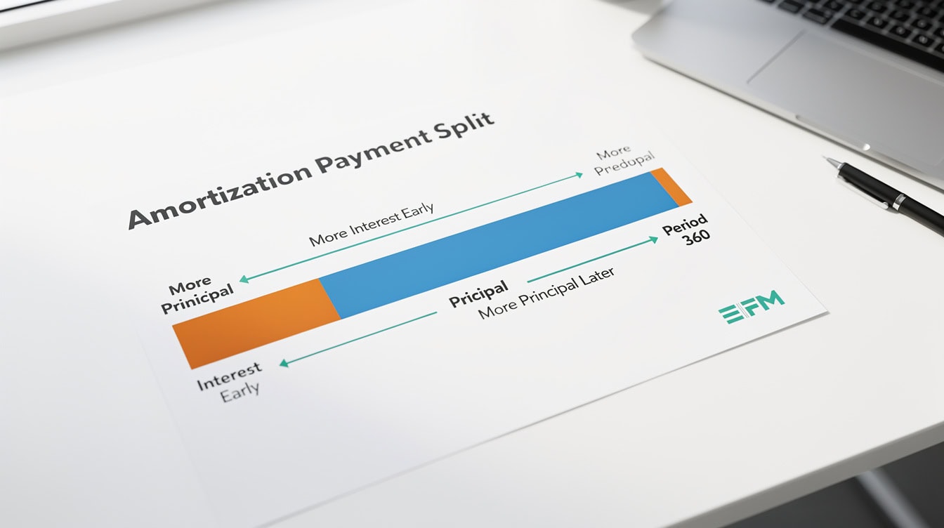
In period 1 of a 30-year mortgage, roughly 86% of each payment covers interest. By period 360, nearly 100% reduces principal.
Essential Components of an Amortization Schedule
Every professional amortization schedule contains six core columns. Each column feeds the next, so the order matters.
| Column | Label | Formula Logic |
|---|---|---|
| A | Period | Sequential integer (1, 2, 3…) |
| B | Beginning Balance | Prior row’s Ending Balance |
| C | Payment | Fixed PMT result |
| D | Interest | Balance × Periodic Rate |
| E | Principal | Payment minus Interest |
| F | Ending Balance | Beginning Balance minus Principal |
You also need a separate input block at the top of the sheet, typically rows 1 through 6, containing the loan amount, annual interest rate, loan term in years, payments per year, and start date. Keeping inputs in named cells (or at minimum in fixed rows) is what allows you to update a single figure and have the entire 360-row schedule recalculate instantly.
Setting Up Your Excel Workbook: Initial Structure and Input Parameters
Before writing a single formula, structure your workbook so inputs are separated from calculations. Place the following in column A (labels) and column B (values) starting at row 1:
- B1: Loan Amount (e.g., 300000)
- B2: Annual Interest Rate (e.g., 0.065)
- B3: Loan Term in Years (e.g., 30)
- B4: Payments Per Year (e.g., 12 for monthly)
- B5: Start Date (e.g., 2024-01-01)
Name these cells using the Name Box (the field left of the formula bar) so you can reference them by name rather than address. Select B1, click the Name Box, type LoanAmount, and press Enter. Repeat for each input. Named ranges make formulas readable and eliminate the risk of accidentally referencing the wrong row.
Row 8 becomes your header row for the schedule table. Enter Period, Beginning Balance, Payment, Interest, Principal, and Ending Balance in columns A through F.
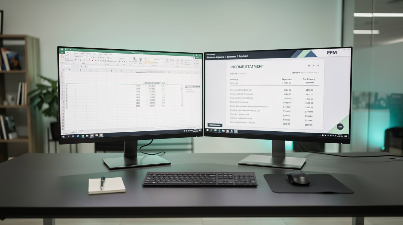
Separating inputs from calculations in a dedicated block is the single most important structural decision in building a dynamic amortization schedule.
Building the Core Formulas: Payment, Interest, and Principal Calculations
The three Excel functions that power every amortization schedule are PMT, IPMT, and PPMT. Each is a built-in financial function (a formula that returns a calculated value based on financial mathematics) that Excel has included since version 5.0.
PMT syntax: =PMT(rate, nper, pv, [fv], type)
rate: periodic interest rate. For monthly payments on a 6.5% annual loan, this isB2/B4or0.065/12.nper: total number of payments. For a 30-year monthly loan, this isB3*B4or360.pv: present value, entered as a negative number to return a positive payment. Use-B1or-LoanAmount.
For the worked example (a $300,000 loan at 6.5% annual rate, 30 years, monthly payments), the PMT formula in cell C2 of your input block is:
=PMT(B2/B4, B3*B4, -B1)
This returns $1,896.20 per month.
IPMT syntax: =IPMT(rate, per, nper, pv)
per: the specific period number for which you want the interest component.
For period 1: =IPMT(0.065/12, 1, 360, -300000) returns $1,625.00.
PPMT syntax: =PPMT(rate, per, nper, pv)
For period 1: =PPMT(0.065/12, 1, 360, -300000) returns $271.20.
Note that $1,625.00 + $271.20 = $1,896.20, confirming the split adds up to the total payment. Excel’s PMT function accepts up to 5 arguments — rate, nper, pv, fv, and type — where the optional fv argument defaults to 0 and the optional type argument defaults to 0 for end-of-period payments.
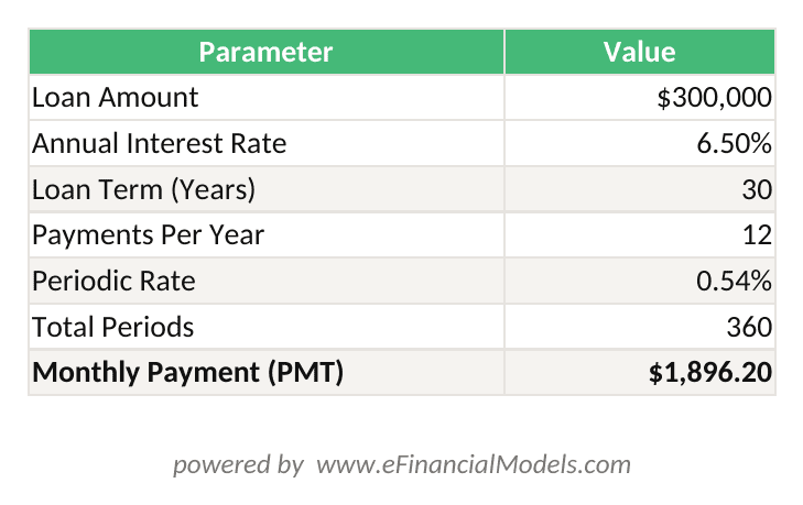
PMT = $1,896.20/month. Period 1 interest = $1,625.00, principal = $271.20. The interest component declines each period as the balance falls.
Constructing the Period-by-Period Schedule with Dynamic Formulas
With inputs defined and core formulas verified, build the schedule row by row starting at row 9 (your first data row, with row 8 as headers).
Row 9 (Period 1):
- A9:
=1 - B9:
=$B$1(beginning balance equals loan amount for period 1; note the absolute reference using$signs, which locks the cell address so it doesn’t shift when you copy the formula down) - C9:
=PMT($B$2/$B$4, $B$3*$B$4, -$B$1)(fixed payment, all absolute references) - D9:
=B9*($B$2/$B$4)(interest = beginning balance × periodic rate) - E9:
=C9-D9(principal = payment minus interest) - F9:
=B9-E9(ending balance = beginning balance minus principal)
Row 10 (Period 2 onward):
- A10:
=A9+1 - B10:
=F9(beginning balance = prior ending balance; this is a relative reference that shifts correctly as you copy down) - C10 through F10: copy the formulas from C9 through F9
Select A10 through F10, then copy and paste down to row 368 (for 360 periods). Because you used absolute references for the input parameters and a relative reference for the beginning balance, every row calculates correctly.
Handling the final payment rounding: The last payment will rarely equal the standard PMT amount exactly due to rounding across 360 periods. Replace the payment formula in the final row (C368) with:
=B368+D368
This sets the final payment to exactly the remaining balance plus one month’s interest, eliminating any residual rounding discrepancy.
Handling Different Payment Frequencies and Compounding Periods
Adjusting for payment frequency requires changing exactly two parameters: the periodic rate and the number of periods. You don’t need separate formulas for monthly, quarterly, or annual schedules.
| Frequency | Payments Per Year (B4) | Periodic Rate | Total Periods |
|---|---|---|---|
| Monthly | 12 | Annual Rate / 12 | Years × 12 |
| Quarterly | 4 | Annual Rate / 4 | Years × 4 |
| Semi-Annual | 2 | Annual Rate / 2 | Years × 2 |
| Annual | 1 | Annual Rate / 1 | Years × 1 |
If your input cell B4 drives the payments-per-year figure, changing B4 from 12 to 4 automatically converts the entire schedule from monthly to quarterly. This is why the dynamic input block matters: one cell change recalculates everything.
A critical distinction: most U.S. mortgages use monthly compounding, meaning the annual rate is simply divided by 12. Canadian mortgages, by contrast, compound semi-annually — as documented by the Bank of Canada — but require monthly payments, which requires converting the stated rate using the formula (1 + annual_rate/2)^(1/6) - 1 to get the true monthly rate.
Always confirm the compounding convention before building a schedule for an international client.

Changing the Payments Per Year input from 12 to 4 converts an entire monthly schedule to quarterly without touching any other formula.
Adding Advanced Features: Extra Payments, Balloon Payments, and Variable Rates
A professional amortization schedule goes beyond the basic structure. Three enhancements cover the most common real-world loan structures.
Extra payments: Add a column G labeled “Extra Payment” where the user can enter an optional additional principal payment for any period. Modify the ending balance formula in F to: =B9-E9-G9. The beginning balance in the next row picks up the reduced balance automatically. Add an IF statement to stop the schedule when the balance reaches zero: =IF(F9<=0, 0, F9).
Balloon payments: A balloon loan (common in commercial real estate) requires a large lump-sum payment at the end of a shorter amortization period. Set the loan term to the full amortization period (say, 30 years) but add an input for the balloon period (say, year 5, or period 60). In the final scheduled row, replace the ending balance with: =IF(A9=BalloonPeriod, 0, B9-E9). The payment in that row becomes the regular PMT plus the remaining balance.
Variable rates: Add a column for the applicable rate in each period. Replace the fixed rate reference in the interest formula with a reference to that column. For an adjustable-rate mortgage (ARM) that resets every 12 periods, use: =IF(MOD(A9,12)=1, NewRate, PriorRate) to trigger the reset at the right intervals.
Validation and Error-Checking: Ensuring Schedule Accuracy
A schedule that looks right but contains a formula error can cost a client real money. Run these four checks before delivering any amortization schedule.
Check 1: Total payments sum. Sum column C (all payments). It should equal the PMT amount multiplied by the number of periods, plus or minus a few cents for rounding. If the difference exceeds $1.00, a formula error exists.
Check 2: Total interest paid. Sum column D. Cross-reference this against the theoretical total interest: (PMT × n) - PV. For the $300,000 example: ($1,896.20 × 360) – $300,000 = $382,632. Your column D sum should match within a dollar.
Check 3: Final ending balance. Cell F368 (the last ending balance) must equal zero or a value within $0.01 of zero. Any larger residual indicates a referencing error in the beginning balance chain.
Check 4: IPMT cross-reference. In a separate cell, calculate =IPMT($B$2/$B$4, 1, $B$3*$B$4, -$B$1) and compare it to D9. They must match exactly. If they don’t, your periodic rate calculation in the schedule is wrong.
Excel supports up to 1,048,576 rows, which comfortably accommodates even a 360-period mortgage schedule with multiple helper columns, so performance is rarely a concern for standard loan schedules.
Common Mistakes and How to Fix Them
These five errors appear repeatedly in amortization schedules built by practitioners at every experience level.
Mistake 1: Not dividing the annual rate by payment frequency. Using B2 instead of B2/B4 as the rate argument in PMT overstates the payment by a factor of 12 for monthly schedules. Fix: always express the rate as a periodic rate.
Mistake 2: Circular references in the beginning balance. If you accidentally reference the current row’s ending balance in the same row’s beginning balance formula, Excel throws a circular reference error (a situation where a formula refers back to its own cell, creating an infinite loop). Fix: the beginning balance in row 10 must reference F9, not F10.
Mistake 3: Mixed absolute and relative references. Copying a formula that uses B2 instead of $B$2 for the interest rate causes the rate reference to shift down one row for each period, producing nonsensical results. Fix: lock all input references with $ before copying.
Mistake 4: Ignoring the final payment rounding. Leaving the standard PMT formula in the last row results in a small negative or positive ending balance. Fix: use the =B368+D368 formula in the final payment cell as described above.
Mistake 5: Rate-period mismatch for non-monthly loans. Using a monthly rate with quarterly periods (or vice versa) produces a schedule that appears to work but generates incorrect interest figures. Fix: always verify that B4 (payments per year) matches the actual payment frequency and that the rate is divided by the same number.
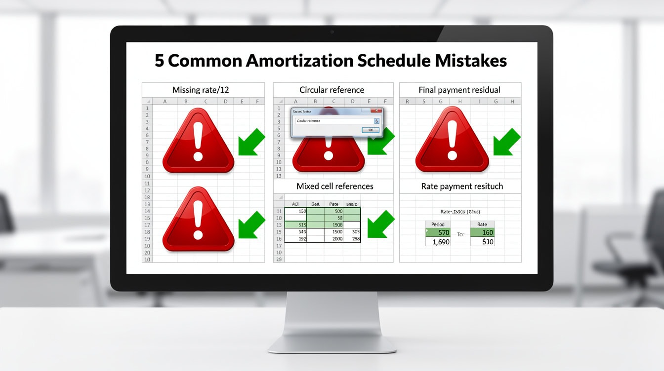
The rate-period mismatch error is the most dangerous because it produces a schedule that looks correct but generates systematically wrong interest figures.
Professional Formatting and Client Presentation Standards
A technically correct schedule that looks like a raw data dump won’t serve a client well. Apply these formatting standards to produce a deliverable that reflects professional financial modeling practice.
Freeze the top rows (View > Freeze Panes > Freeze Top Row) so column headers remain visible while scrolling through 360 periods. Format currency columns (B, C, D, E, F) as accounting format with 2 decimal places. Apply conditional formatting to highlight any row where the ending balance drops below zero in red, which immediately flags an extra-payment scenario that has overpaid the loan.
For print output, set the print area to the schedule table, enable “Repeat Rows at Top” (Page Layout > Print Titles) so headers appear on every printed page, and set column widths so the schedule fits on a standard 8.5 × 11 page in landscape orientation. The EFM debt schedule templates follow these conventions and include pre-built print settings.
For client-facing models, add a summary box above the schedule showing: loan amount, monthly payment, total interest paid, total amount paid, and effective annual cost. These five figures answer the questions every borrower or lender asks first.
A client-ready schedule leads with the five numbers every borrower asks about before presenting the full period-by-period detail.
Practical Applications Across Loan Types and Financial Products
The same Excel structure applies across loan types, but the input parameters differ significantly. Understanding these differences prevents you from applying mortgage conventions to a commercial loan or vice versa.
| Loan Type | Typical Term | Typical Rate | Payment Freq | Key Difference |
|---|---|---|---|---|
| Residential Mortgage | 15-30 years | 6-8% (2024) | Monthly | Escrow for taxes/insurance |
| Auto Loan | 48-84 months | 5-10% | Monthly | Simple interest, no compounding |
| Business Term Loan | 1-10 years | 7-12% | Monthly/Quarterly | Origination fees affect APR |
| Equipment Financing | 3-7 years | 6-10% | Monthly | Residual/balloon common |
| Commercial Real Estate | 5-25 years | 6-9% | Monthly | Balloon at 5-10 years typical |
For commercial real estate loans, the amortization period and the loan term are often different: a loan might amortize over 25 years but have a 10-year balloon, meaning the borrower makes payments as if the loan runs 25 years but must refinance or pay off the remaining balance at year 10. The EFM commercial real estate Excel model handles this structure with built-in balloon payment logic.
For business planning purposes, the amortization schedule feeds directly into the cash flow statement (principal payments are financing outflows, not operating expenses) and the balance sheet (the ending balance each period is the loan liability). Analysts building integrated three-statement models need the schedule to link correctly to both statements. The EFM debt amortization templates include these linkages pre-built.
The U.S. Small Business Administration reports that term loans remain the most common form of small business financing, which means amortization schedules are a daily tool for accountants, CFOs, and financial analysts serving the small business market.
Frequently Asked Questions
What is the difference between PMT, IPMT, and PPMT in Excel?
PMT calculates the total fixed periodic payment for a loan. IPMT (Interest Payment) returns only the interest portion of a specific payment in a given period. PPMT (Principal Payment) returns only the principal portion for a specific period. For example, on a $300,000 loan at 6.5% annual rate over 30 years, =PMT(0.065/12, 360, -300000) returns $1,896.20, while =IPMT(0.065/12, 1, 360, -300000) returns $1,625.00 and =PPMT(0.065/12, 1, 360, -300000) returns $271.20. The IPMT and PPMT values always sum to the PMT value for any given period. Use IPMT and PPMT for spot-checking individual rows in your schedule without building the full table.
Why does my amortization schedule show a small balance remaining after the last payment?
This happens because Excel rounds each payment to 2 decimal places, and those rounding differences accumulate across hundreds of periods. On a 360-period schedule, the residual is typically between $0.01 and $0.50. The fix is to replace the PMT formula in the final row with =B368+D368, which sets the last payment to exactly the remaining balance plus one period’s interest. This is standard practice in professional financial modeling and matches how lenders actually handle final payments. Never ignore a residual larger than $1.00, as that indicates a formula error rather than a rounding issue.
How do I adjust my amortization schedule for quarterly or annual payments instead of monthly?
Change the Payments Per Year input (B4) from 12 to 4 (quarterly) or 1 (annual). The PMT formula =PMT(B2/B4, B3*B4, -B1) automatically adjusts because both the periodic rate (B2/B4) and the total periods (B3B4) recalculate. For a $300,000 loan at 6.5% over 30 years with quarterly payments, the formula becomes `=PMT(0.065/4, 120, -300000)`, returning $5,765.82 per quarter. The total interest paid will differ slightly from the monthly version because interest compounds at a different frequency. Always verify that your payment frequency matches the loan agreement before presenting the schedule to a client.
How do I add extra payment functionality to my amortization schedule?
Add a column G labeled “Extra Payment” where users can enter optional additional principal payments for any period. Modify the ending balance formula in column F from `=B9-E9` to `=MAX(B9-E9-G9, 0)`. The MAX function prevents the balance from going negative if an extra payment exceeds the remaining principal. Update the beginning balance formula in the next row to reference the new ending balance. Add a conditional check so the schedule stops calculating once the balance reaches zero: wrap the payment formula in `=IF(B9=0, 0, PMT(…))`. This structure lets you model the interest savings from making extra principal payments, which is one of the most common client requests in personal finance planning.
What validation checks should I run before sending an amortization schedule to a client?
Run four checks. First, confirm the sum of all payments in column C equals PMT × n within $1.00. Second, verify the sum of all interest payments in column D equals (PMT × n) – PV within $1.00; for the $300,000 example, total interest should be approximately $382,632. Third, confirm the final ending balance in column F equals zero or within $0.01 of zero. Fourth, cross-reference the period 1 interest figure in D9 against `=IPMT(rate/periods, 1, nper, -pv)` calculated independently; they must match exactly. If any check fails, trace the error back to the beginning balance chain or the rate-period calculation before delivering the file.
Can I build an amortization schedule for a loan with a balloon payment in Excel?
Yes. A balloon payment loan amortizes over a longer period (say, 30 years) but requires full repayment at an earlier date (say, year 5, or period 60). Build the full 360-row schedule using the standard 30-year PMT. Then, in the row corresponding to the balloon period (row 68 for period 60), replace the ending balance formula with `=IF(A68=BalloonPeriod, 0, B68-E68)` and replace the payment formula with `=B68(1+$B$2/$B$4)` to capture the full payoff. The schedule will show 59 regular payments followed by one large balloon payment that retires the remaining balance. This structure is standard in commercial real estate financing, where 5- and 10-year balloons on 25- or 30-year amortization schedules are common.
How does an amortization schedule connect to a three-statement financial model?
The amortization schedule feeds two of the three financial statements. The interest expense from column D flows to the income statement as a financing cost, reducing pre-tax income. The principal repayment from column E flows to the cash flow statement under financing activities as a cash outflow (not an operating expense). The ending balance from column F flows to the balance sheet as the current loan liability at each period end. In a properly linked model, changing the loan amount or interest rate in the amortization schedule automatically updates all three statements. The EFM general Excel financial models include pre-linked debt schedules that demonstrate this integration.
Conclusion
Building an amortization schedule in Excel is a foundational financial modeling skill that pays dividends across mortgage analysis, business loan structuring, commercial real estate underwriting, and client advisory work. The PMT, IPMT, and PPMT functions handle the mathematics; absolute cell references make the schedule dynamic; and the four validation checks confirm accuracy before any number reaches a client’s desk.
I recommend downloading the EFM professional amortization schedule template to get a pre-built, validated schedule with extra payment functionality, balloon payment toggles, and client-ready formatting already in place, so you can focus on the analysis rather than the construction.