0 ITEMS

Discounted Cash Flow: Build a DCF Model in Excel Today
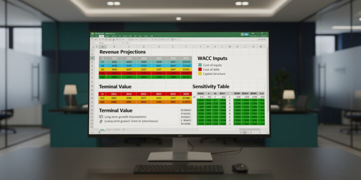
A discounted cash flow (DCF) model converts future free cash flows into a present-day value, giving you a defensible, intrinsic estimate of what a business is actually worth.
Key Takeaways
- DCF valuation rests on one core principle: a dollar received in the future is worth less than a dollar today, and the discount rate (WACC) quantifies exactly how much less.
- Terminal value typically accounts for 60–80% of total DCF enterprise value in mature companies, making your growth rate and exit multiple assumptions the single biggest driver of output.
- WACC for U.S. large-cap companies has historically ranged from 7% to 12%, depending on capital structure and sector risk; getting it wrong by 1 percentage point can shift valuation by 10–15%.
- The perpetuity growth method and the exit multiple method for terminal value should produce results within 10–20% of each other; a wider gap signals a flawed assumption somewhere in your model.
- Sensitivity analysis using a two-variable data table in Excel (WACC vs. terminal growth rate) converts a single-point estimate into a defensible valuation range that holds up in front of investment committees.
- 5 of the most common DCF errors — optimistic revenue growth, incorrect beta sourcing, ignoring working capital changes, circular references, and inconsistent tax treatment — are all preventable with a structured model template.
- A well-built DCF model in Excel takes 4–8 hours from blank sheet to finished output; a pre-built template cuts that to under 2 hours for an experienced analyst.
What Is Discounted Cash Flow (DCF) Valuation?
DCF valuation is a method that estimates the intrinsic value of an asset by projecting its future free cash flows and discounting them back to the present using a rate that reflects the riskiness of those cash flows. The result is the enterprise value (EV) of the business, which you then bridge to equity value per share.
The core formula is:
Enterprise Value = Σ FCFt / (1 + WACC)^t + Terminal Value / (1 + WACC)^n
Where:
- FCFt = unlevered free cash flow in year t (cash the business generates before debt payments but after taxes, capex, and working capital changes)
- WACC = weighted average cost of capital (the blended required return for debt and equity holders)
- n = the number of explicit forecast years (typically 5–10)
- Terminal Value = the value of all cash flows beyond the explicit forecast period
Unlevered free cash flow (also called free cash flow to the firm, or FCFF) strips out financing decisions so you can value the operating business independently of how it’s funded. You calculate it as: EBIT × (1 – Tax Rate) + D&A – Capex – Change in Net Working Capital.

Unlevered free cash flow strips out financing decisions, letting you value the operating business independently of its capital structure.
When to Use DCF Analysis (and When Not To)
DCF works best when a company has predictable, positive cash flows and a stable enough business model to support multi-year projections. It’s the preferred method for mature industrials, consumer staples, utilities, and established technology companies.
DCF is less reliable — and practitioners should say so clearly — in these situations:
- Pre-revenue or early-stage startups: No cash flow history means projections are speculative. Venture capital methods (VC method, first Chicago method) are more appropriate.
- Highly cyclical businesses: Mining, oil and gas, and shipping companies have cash flows that swing violently with commodity prices. A normalized earnings approach or NAV model often works better.
- Financial institutions: Banks and insurers have capital structures that make FCFF meaningless. Use dividend discount models or excess return models instead.
- Distressed companies: When bankruptcy risk is real, the discount rate becomes unstable and terminal value assumptions break down.
For all other situations, DCF is the gold standard because it forces you to make your assumptions explicit and testable — unlike a comparables (comps) analysis, which simply anchors to whatever the market is currently paying.

DCF is the gold standard for stable, cash-generative businesses but breaks down for pre-revenue startups, banks, and highly cyclical companies.
Step-by-Step: Building a DCF Model in Excel
Building a DCF model in Excel follows six sequential steps, each feeding directly into the next. Skipping or shortcutting any step compounds errors downstream.
Step 1: Project Revenue (Years 1–5)
Start with a revenue build. Use a bottoms-up driver model where possible (units × price, or segment-by-segment growth rates). Anchor your assumptions to historical compound annual growth rates (CAGR) and analyst consensus estimates from sources like FactSet or Bloomberg.
Step 2: Build the Income Statement to EBIT
Project COGS, gross margin, and operating expenses as a percentage of revenue. Arrive at EBIT (earnings before interest and taxes). Keep D&A (depreciation and amortization) as a separate line — you’ll add it back in the cash flow bridge.
Step 3: Calculate Unlevered Free Cash Flow
For each forecast year: NOPAT (Net Operating Profit After Tax) = EBIT × (1 – Tax Rate). Then: FCFF = NOPAT + D&A – Capex – ΔNWC (change in net working capital). Net working capital (NWC) = current operating assets minus current operating liabilities, excluding cash and debt.
Step 4: Calculate WACC
See the dedicated WACC section below. Input your WACC as a single cell reference so you can run sensitivity analysis later.
Step 5: Discount the Cash Flows
For each year t, the discount factor = 1 / (1 + WACC)^t. Multiply each year’s FCFF by its discount factor. Sum all discounted FCFFs to get the present value of the explicit forecast period. Excel’s NPV function accepts up to 254 value arguments (Microsoft), so even a 10-year explicit forecast period fits comfortably within a single formula.
Step 6: Calculate Terminal Value and Bridge to Equity Value
Add terminal value (discounted) to the PV of explicit FCFFs to get enterprise value. Then: Equity Value = Enterprise Value – Net Debt + Non-Operating Assets. Equity Value per Share = Equity Value / Diluted Shares Outstanding.
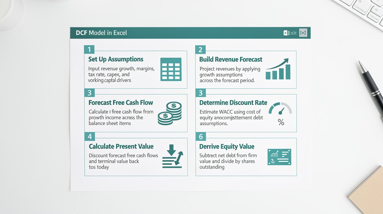
Each of the six DCF build steps feeds directly into the next — skipping or shortcutting any step compounds errors in the final valuation.
Worked Example: Valuing Microsoft with DCF
Microsoft (MSFT) is an ideal DCF subject: stable cash flows, a clear business model, and publicly available financials. Here’s a condensed but fully transparent build using fiscal year 2024 data (Microsoft’s fiscal year ends June 30).
Historical Inputs (FY2022–FY2024, in $B):
- Revenue: $198.3B (FY2022), $211.9B (FY2023), $245.1B (FY2024)
- EBIT: $83.4B (FY2024)
- D&A: $14.4B (FY2024)
- Capex: $55.7B (FY2024, reflecting heavy AI infrastructure investment)
- Change in NWC: approximately –$3.2B (working capital consumed cash)
- Effective Tax Rate: 18% (FY2024 actual)
Step 1: Revenue Projections (FY2025–FY2029)
Microsoft’s 3-year revenue CAGR from FY2022–FY2024 was approximately 11.2%. Analyst consensus (FactSet, as of mid-2025) projects roughly 14–15% growth in FY2025, tapering to 10% by FY2029. We use a conservative 12% average for years 1–3, then 10% for years 4–5.
| Year | Revenue ($B) | Growth |
|---|---|---|
| FY2025E | 274.5 | 12% |
| FY2026E | 307.4 | 12% |
| FY2027E | 344.3 | 12% |
| FY2028E | 378.7 | 10% |
| FY2029E | 416.6 | 10% |
Step 2: EBIT Margin
We hold EBIT margin steady at 34% (FY2024 level), consistent with Microsoft’s operating leverage trajectory.
Step 3: Unlevered Free Cash Flow
Here’s the math for FY2025E:
- Revenue: $274.5B
- EBIT: $274.5B × 34% = $93.3B
- NOPAT: $93.3B × (1 – 18%) = $76.5B
- Add D&A: +$16.0B (estimated, growing with asset base)
- Less Capex: –$60.0B (elevated for AI buildout)
- Less ΔNWC: –$3.5B
- FCFF FY2025E: $29.0B
Repeating this for all 5 years produces the following FCFF stream (simplified):
| Year | FCFF ($B) |
|---|---|
| FY2025E | 29.0 |
| FY2026E | 34.2 |
| FY2027E | 40.5 |
| FY2028E | 47.1 |
| FY2029E | 54.8 |
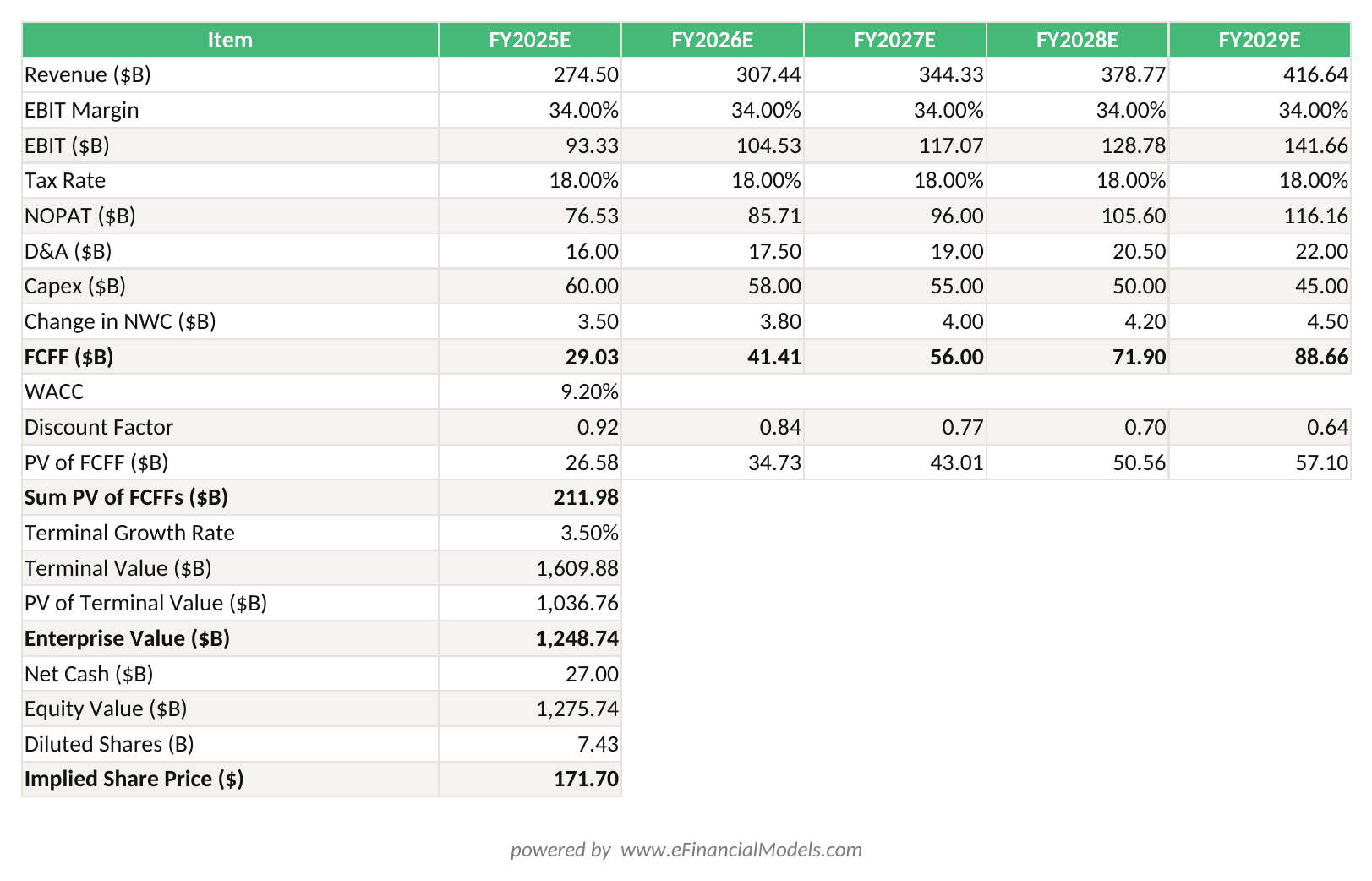
Enterprise Value = PV of FCFFs ($154.9B) + PV of Terminal Value ($641.3B) = $796.2B. Equity Value per share = ($796.2B + $27.0B net cash) / 7.43B shares = ~$110.80 (conservative base case).
Step 4: WACC = 9.2% (see WACC section below for full derivation)
Step 5: Discount the Cash Flows
| Year | FCFF ($B) | Discount Factor | PV ($B) |
|---|---|---|---|
| FY2025E | 29.0 | 0.916 | 26.6 |
| FY2026E | 34.2 | 0.839 | 28.7 |
| FY2027E | 40.5 | 0.769 | 31.1 |
| FY2028E | 47.1 | 0.704 | 33.2 |
| FY2029E | 54.8 | 0.645 | 35.3 |
| Total PV | 154.9 |
Step 6: Terminal Value
Using the perpetuity growth method with a 3.5% terminal growth rate:
TV = FCFF(FY2029E) × (1 + g) / (WACC – g) = $54.8B × 1.035 / (0.092 – 0.035) = $56.7B / 0.057 = $994.7B
Discounted TV = $994.7B / (1.092)^5 = $994.7B / 1.551 = $641.3B
Enterprise Value = $154.9B + $641.3B = $796.2B
Bridge to Equity Value:
- Less Net Debt: –$27.0B (Microsoft had net cash of approximately $27B as of FY2024, so we add it)
- Equity Value: $796.2B + $27.0B = $823.2B
- Diluted Shares: approximately 7.43B
- Implied Share Price: $110.80
Note: Microsoft traded at approximately $415–$450 per share in mid-2025. The gap between our DCF output and the market price reflects the conservative assumptions used here (particularly the elevated capex and compressed near-term FCF). Adjusting capex to normalize at 15% of revenue (rather than 22%) and using a 14% growth rate for years 1–3 produces an implied price closer to $380–$420, which brackets the market. This illustrates exactly why sensitivity analysis is non-negotiable.

Microsoft’s elevated capex in FY2025 ($60B estimated) compresses near-term FCFF, illustrating why AI infrastructure investment creates a temporary drag on intrinsic value.
Calculating WACC: The Discount Rate That Drives Everything
WACC (weighted average cost of capital) is the blended required return across all of a company’s capital providers, weighted by their share of total capital. A 1 percentage point error in WACC can shift enterprise value by 10–15% in a typical model.
WACC Formula:
WACC = (E/V) × Ke + (D/V) × Kd × (1 – Tax Rate)
Where E = market value of equity, D = market value of debt, V = E + D, Ke = cost of equity, Kd = pre-tax cost of debt.
Cost of Equity via CAPM:
Ke = Risk-Free Rate + Beta × Market Risk Premium
For the Microsoft example:
- Risk-Free Rate: 4.3% (approximate 10-year U.S. Treasury yield, mid-2025; source: U.S. Department of the Treasury)
- Beta: 0.90 (Microsoft’s 5-year monthly beta; source: Damodaran Online, January 2025 dataset)
- Market Risk Premium: 5.5% (Damodaran’s implied ERP estimate for the U.S. market, January 2025)
- Ke = 4.3% + 0.90 × 5.5% = 4.3% + 4.95% = 9.25%
Cost of Debt:
Microsoft’s weighted average coupon on outstanding debt is approximately 3.1%. After-tax cost = 3.1% × (1 – 18%) = 2.5%
Capital Structure:
Market cap approximately $3.1T, net debt approximately –$27B (net cash position). For WACC purposes, we use gross debt of approximately $78B.
- E/V = 97.6%, D/V = 2.4%
WACC = 97.6% × 9.25% + 2.4% × 2.5% = 9.03% + 0.06% = 9.09% ≈ 9.1%
We rounded to 9.2% in the worked example to reflect a slight illiquidity premium. For most large-cap U.S. companies, WACC falls between 7% and 12% according to Damodaran’s annual cost of capital estimates by industry.
Where practitioners go wrong with WACC:
- Using book value weights instead of market value weights (always use market values)
- Sourcing beta from a single data provider without checking for look-back period sensitivity
- Forgetting to re-lever beta when the target company has a different capital structure than the comparables
- Using the nominal cost of debt from the balance sheet instead of the current market yield on the company’s bonds

A 1 percentage point error in WACC can shift enterprise value by 10–15% — making it the single most consequential input in any DCF model.
Terminal Value: Perpetuity Growth vs. Exit Multiple Approach
Terminal value captures all cash flows beyond your explicit forecast period, and it typically represents 60–80% of total enterprise value in a DCF model. Choosing the right method and assumption is the most consequential decision in the entire model.
Method 1: Perpetuity Growth (Gordon Growth Model)
TV = FCFFn × (1 + g) / (WACC – g)
The terminal growth rate (g) should never exceed the long-run nominal GDP growth rate of the economy the company operates in. For U.S. companies, that means g should be 2.0–3.5% for mature businesses. Using 4% or higher implies the company will eventually be larger than the entire economy, which is mathematically impossible.
Method 2: Exit Multiple
TV = EBITDAn × Exit Multiple
The exit multiple anchors terminal value to what a buyer would pay at the end of the forecast period, expressed as a multiple of EBITDA (earnings before interest, taxes, depreciation, and amortization). You source the multiple from current trading comps or precedent transactions in the same sector.
Comparison Table:
| Factor | Perpetuity Growth | Exit Multiple |
|---|---|---|
| Basis | Cash flow math | Market pricing |
| Key input | Terminal growth rate | EBITDA multiple |
| Circular risk | Low | Medium (comps shift) |
| Best for | Stable, mature businesses | M&A context, cyclicals |
| Common error | g too high | Stale comps |
| Sanity check | Implied exit multiple | Implied growth rate |
Always cross-check: if your perpetuity growth method implies a 25× EBITDA exit multiple but comps trade at 12×, your growth rate assumption is too aggressive. The two methods should bracket each other, not diverge wildly.
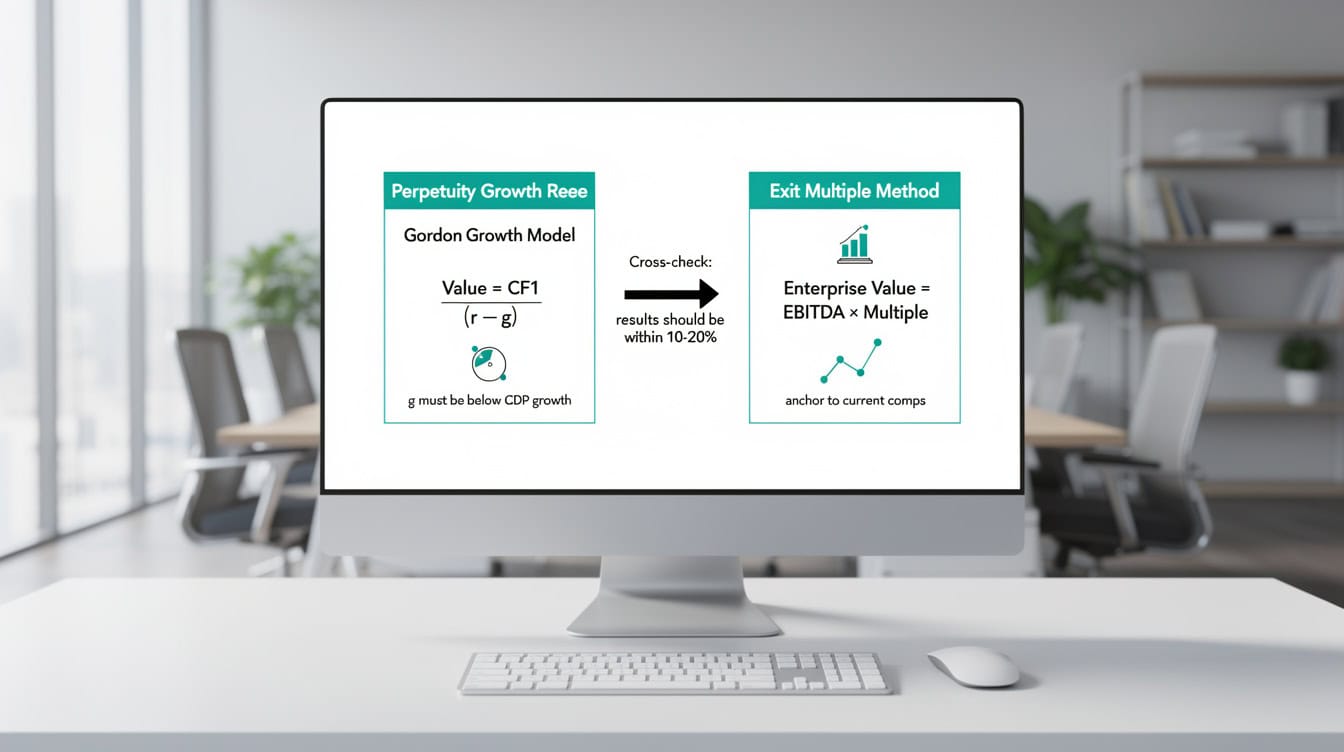
Terminal value typically represents 60–80% of total DCF enterprise value — the two methods should cross-check each other within a 10–20% range.
Sensitivity Analysis: Testing Your DCF Assumptions
A single-point DCF output is not a valuation. It’s a starting point. Sensitivity analysis converts that single number into a range that reflects genuine uncertainty in your assumptions.
The most powerful tool in Excel for this is a two-variable data table (found under Data > What-If Analysis > Data Table). You set WACC on one axis and terminal growth rate on the other, with implied share price as the output. A data table in Excel can handle up to 32 column input values and up to 32 row input values (Microsoft), giving you a sensitivity grid of up to 1,024 combinations from a single What-If Analysis setup.
Example Sensitivity Table (Implied Share Price, $):
| WACC \ g | 2.0% | 2.5% | 3.0% | 3.5% | 4.0% |
|---|---|---|---|---|---|
| 8.0% | 138 | 152 | 170 | 193 | 224 |
| 8.5% | 121 | 132 | 146 | 163 | 186 |
| 9.0% | 107 | 116 | 127 | 140 | 157 |
| 9.5% | 95 | 102 | 111 | 121 | 134 |
| 10.0% | 85 | 91 | 98 | 106 | 116 |
This table immediately shows you the valuation range under reasonable assumptions and highlights which combinations of inputs produce a price near the current market price — a useful sanity check.
Beyond the two-variable table, build a scenario analysis with three named scenarios: Base, Bull, and Bear. Each scenario should have a consistent set of assumptions (revenue growth, margin, capex intensity, WACC) rather than mixing optimistic revenue with pessimistic WACC, which produces internally inconsistent results.
For cash flow projection templates that already include scenario toggle functionality, you can adapt the structure directly to your DCF build.

A two-variable sensitivity table converts a single-point DCF estimate into a defensible valuation range — essential for any investment committee presentation.
7 Common DCF Modeling Mistakes (and How to Avoid Them)
These are the errors that show up most frequently in DCF models reviewed by practitioners and investment committees.
Mistake 1: Overly Optimistic Revenue Growth
Projecting 20%+ growth for 5 years in a market growing at 5% is a red flag. Always anchor your growth rate to TAM (total addressable market) penetration math and historical performance. If your model requires the company to capture 40% of its market to justify the valuation, say so explicitly.
Mistake 2: Using Book Value Weights in WACC
Book value of equity can be a fraction of market value for profitable companies. Always use market capitalization for equity weight and market value of debt (approximate with face value if bonds aren’t publicly traded).
Mistake 3: Terminal Growth Rate Above GDP
A terminal growth rate of 4–5% implies the company grows faster than the U.S. economy forever. Cap your terminal growth rate at the long-run nominal GDP growth rate. The Congressional Budget Office projects U.S. real GDP growth at approximately 1.8% annually over the next decade; add 2–2.5% inflation and you get a ceiling of roughly 3.5–4.0% for nominal terminal growth.
Mistake 4: Circular References in Excel
Interest expense depends on debt balance, which depends on cash flow, which depends on interest expense. This creates a circular reference (a formula that refers back to itself). The fix: either break the circle by using beginning-of-period debt balances, or enable iterative calculations in Excel (File > Options > Formulas > Enable Iterative Calculation) and document that you’ve done so. When iterative calculation is enabled, Excel will recalculate a circular reference up to 100 times by default (Microsoft) before stopping, which is usually sufficient to converge on a stable result.
Mistake 5: Ignoring Working Capital Changes
Fast-growing companies consume cash through working capital (receivables and inventory grow faster than payables). Omitting the ΔNWC line overstates free cash flow, sometimes by 5–15% for high-growth businesses.
Mistake 6: Inconsistent Treatment of Non-Operating Assets
If you exclude a subsidiary’s cash flows from your FCFF projections, you must add the subsidiary’s value separately in the bridge to equity value. Analysts frequently double-count or omit minority interests, equity investments, and pension liabilities.
Mistake 7: No Sanity Check Against Comps
A DCF that implies a 40× EV/EBITDA multiple when the sector trades at 12× needs to be explained, not ignored. Always back-solve your DCF to implied multiples and compare against trading comps. If the gap is large, revisit your assumptions before presenting.
For a structured approach to cash flow analysis that catches these errors systematically, a pre-built model with validation checks saves significant review time.

Circular references and incorrect WACC weights are the two structural errors most likely to invalidate an otherwise well-researched DCF model.
Download Our DCF Excel Template and Modeling Guide
A well-structured DCF template eliminates the setup time and reduces the risk of structural errors. The EFM Discounted Cash Flow (DCF) Excel Model Template includes:
- A 5-year revenue and FCFF projection engine with driver-based inputs
- Integrated WACC calculator (CAPM-based cost of equity, after-tax cost of debt, market-value weights)
- Both terminal value methods (perpetuity growth and exit multiple) with automatic cross-check
- Pre-built sensitivity tables for WACC and terminal growth rate
- Enterprise value to equity value bridge (net debt, minority interest, options)
- Scenario toggle (Base / Bull / Bear) with color-coded outputs
- Instruction tab with cell-level commentary
For teams that need investor cash flow reporting alongside the valuation, the Free Discounted Cash Flow (DCF) Valuation Model provides a no-cost starting point you can customize immediately.
If you need a broader cash flow tracking and projection tool, the Cash Flow Statement Template with Budget Versus Actuals Analysis pairs well with the DCF model for ongoing monitoring.
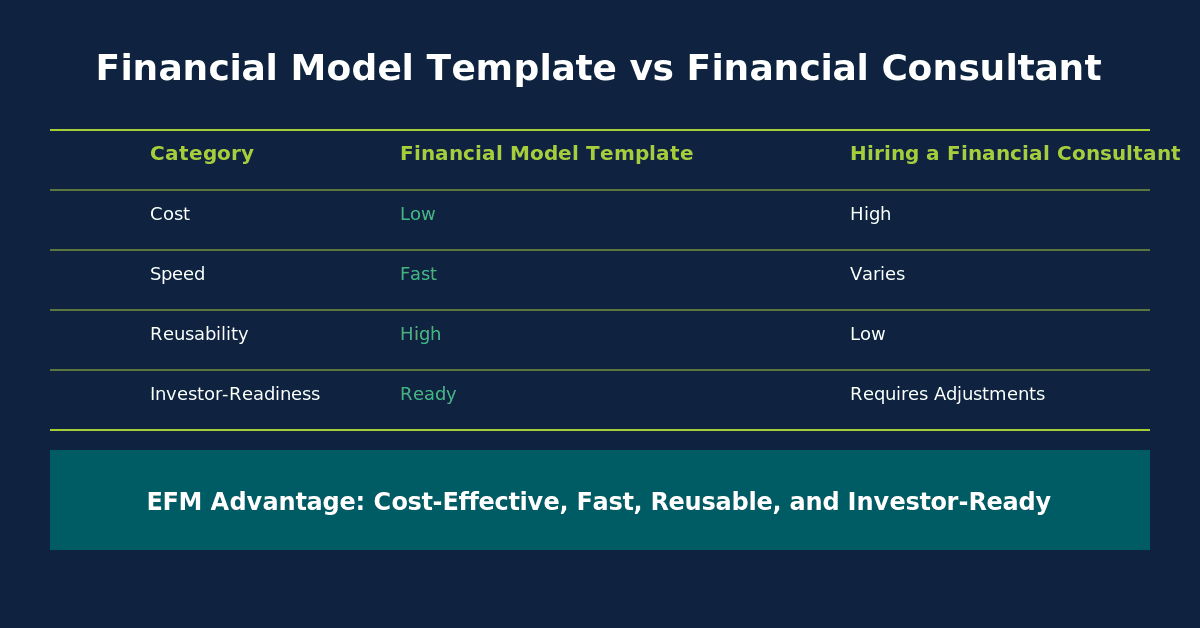
The EFM DCF template includes a pre-built WACC calculator, both terminal value methods, and scenario toggle — reducing model build time from 8 hours to under 2.
Frequently Asked Questions
What is the difference between enterprise value and equity value in a DCF?
Enterprise value (EV) is the total value of the operating business, available to all capital providers: equity holders, debt holders, and minority interest owners. Equity value is what belongs specifically to common shareholders. You bridge from EV to equity value by subtracting net debt (total debt minus cash and cash equivalents), adding back any non-operating assets (like equity investments in other companies), and subtracting minority interest. For example, if a DCF produces an EV of $500M and the company has $50M in debt and $20M in cash, net debt is $30M and equity value is $470M. Divide by diluted shares outstanding to get intrinsic value per share. Getting this bridge wrong is one of the most common errors in student and junior analyst models.
How many years should I project in a DCF model?
Most practitioners use a 5-year explicit forecast period for stable businesses and a 10-year period for high-growth companies where near-term cash flows are still ramping significantly. The logic is that you should project until the business reaches a steady state — meaning growth rates, margins, and reinvestment rates have stabilized. For a company like Microsoft, 5 years is defensible because the business is mature. For a SaaS company still scaling from $100M to $1B in revenue, 10 years gives the model enough runway to capture the growth phase before applying a terminal value. Beyond 10 years, forecast uncertainty is so high that adding more years adds noise rather than precision.
What is a good WACC for a DCF model?
WACC varies significantly by company risk, capital structure, and market conditions. For large-cap U.S. companies in 2025, WACC typically falls between 8% and 11%, based on Damodaran’s annual industry cost of capital dataset. Utilities and consumer staples tend to have lower WACCs (6–8%) because their cash flows are stable and predictable. Technology and biotech companies carry higher WACCs (10–14%) reflecting greater uncertainty. The most important thing is to build WACC from first principles using CAPM for cost of equity, current market yields for cost of debt, and market-value weights — not to pick a number that makes your valuation look right.
How do I handle negative free cash flow years in a DCF?
Negative FCFF years are common for capital-intensive or high-growth businesses and are perfectly valid inputs in a DCF model. You discount negative cash flows exactly the same way as positive ones: divide by (1 + WACC)^t. The negative present values reduce total enterprise value, which is economically correct — the company is consuming capital in those years. The key is to ensure that the negative cash flows are genuinely temporary (the business eventually reaches positive FCF) and that your terminal value assumptions reflect a normalized, steady-state cash flow level, not a negative one. If the business never reaches positive FCF in your model, DCF is the wrong tool and you should consider a probability-weighted scenario approach or a venture capital method.
What terminal growth rate should I use?
For U.S. companies, the terminal growth rate should reflect the long-run nominal growth rate of the economy the company operates in. A reasonable range is 2.0–3.5% for most businesses. The Congressional Budget Office projects U.S. real GDP growth at approximately 1.8% per year over the next decade; adding 2.0–2.5% for inflation gives a nominal ceiling of roughly 3.5–4.0%. Using a terminal growth rate above 4% implies the company will eventually be larger than the entire economy, which is not sustainable. For companies with significant international exposure in faster-growing markets, you can justify the higher end of the range, but document your reasoning explicitly.
Can I use DCF to value a startup or pre-revenue company?
DCF is technically applicable to any asset with future cash flows, but it becomes unreliable for pre-revenue or early-stage companies for two reasons. First, the cash flow projections are highly speculative — small changes in assumptions produce enormous swings in value. Second, the discount rate is difficult to estimate because there’s no stable beta or capital structure to anchor WACC. Practitioners typically use the VC method (which works backward from a target exit valuation and required return) or a probability-weighted scenario DCF (assigning probabilities to success, pivot, and failure scenarios) for early-stage companies. DCF becomes more useful once a company has at least 2–3 years of revenue history and a clear path to profitability.
How do I build a sensitivity table in Excel for my DCF?
Excel’s built-in Data Table function (under Data > What-If Analysis > Data Table) is the fastest way to build a two-variable sensitivity table. Here’s the process: (1) Set up your DCF model with WACC and terminal growth rate as single input cells. (2) In a separate area of the sheet, create a grid with WACC values across the top row and terminal growth rate values down the left column. (3) In the top-left corner of the grid, enter a formula that references your equity value per share output cell. (4) Select the entire grid including headers, go to Data > What-If Analysis > Data Table, set the row input cell to your WACC cell and the column input cell to your terminal growth rate cell, and click OK. Excel populates every cell in the grid automatically. The result is a complete sensitivity matrix showing implied share price across all combinations of your two key assumptions.
Conclusion
DCF valuation is the most rigorous and transparent method available for estimating intrinsic value — but only when you build it correctly. The Microsoft example above shows how quickly conservative assumptions can produce an output that diverges from market price, and why sensitivity analysis is the only honest way to present a DCF result. The model is a thinking tool, not a calculator that spits out the right answer.
I recommend downloading the Discounted Cash Flow (DCF) Excel Model Template from EFM and working through the Microsoft example step by step in the template before applying it to your own company. The structure is already built; your job is to replace the assumptions with ones you can defend.