0 ITEMS

Levered vs. Unlevered IRR: A Practical Framework
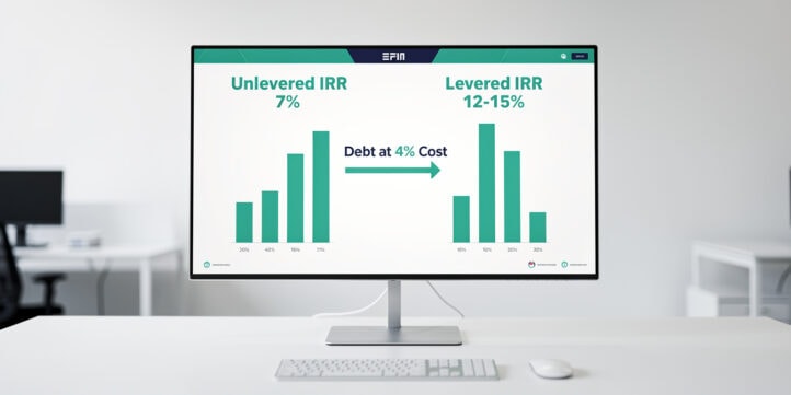
A deal financed with 90% debt can post a 30% levered IRR while the underlying asset earns just 7.7% on its own — a gap that looks like skill but is pure financial engineering. Knowing how to separate levered from unlevered IRR is what tells you whether you’re buying a genuinely good asset or just borrowing your way to an attractive-looking number.
Key Takeaways
- Unlevered IRR measures an asset’s standalone return with zero debt; levered IRR measures the equity return after debt service, and the two diverge sharply as loan-to-value (LTV) rises.
- A property with a 7% unlevered return and 4% debt cost produces a 12% levered IRR at 60% LTV and a 15% levered IRR at 75% LTV, according to BubbleGumBI — a near-doubling of the headline return from financing alone.
- Leverage adds value only when the debt cost sits below the unlevered IRR; when debt cost exceeds unlevered IRR, every dollar of borrowing destroys equity value.
- Unlevered IRR isolates asset quality from financing decisions, making it the correct metric for comparing deals with different capital structures.
- Levered IRR has four components: initial equity investment, annual equity cash flows, any refinance proceeds, and exit sale proceeds.
- The beta analogy is direct: levered beta spans roughly 1.10 to 1.55 in a typical comparable set, while unlevered beta compresses to 0.96 to 1.05 after stripping out capital structure effects.
- Always verify that unlevered IRR exceeds WACC before relying on leverage to hit your return target — otherwise you are engineering returns on a fundamentally weak asset.
Private equity analysts and real estate investors face the same trap: a deal with 90% debt financing can show a 30% levered IRR while the underlying asset earns only 7.7% on its own. That gap is not alpha — it is financial engineering. Understanding levered vs. unlevered IRR is how you tell the difference.
Defining Levered and Unlevered IRR
Levered IRR is the discount rate at which the net present value (NPV) of all equity cash flows equals zero, meaning it measures the return to equity holders after accounting for debt service. Unlevered IRR, by contrast, treats the investment as if it were purchased entirely with equity, capturing the asset’s pure operating return before any financing effects.
The internal rate of return (IRR) itself is the rate r that solves:
0 = CF₀ + CF₁/(1+r) + CF₂/(1+r)² + … + CFₙ/(1+r)ⁿ
Swap in unlevered free cash flows (cash flows available to all capital providers) and you get the unlevered IRR, also called the Project IRR. Swap in levered free cash flows (cash flows available to equity holders only) and you get the levered IRR, also called the Equity IRR. According to BubbleGumBI, levered IRR is specifically the rate at which the NPV of all equity cash flows equals zero.
Unlevered free cash flow (UFCF) is calculated as:
UFCF = EBIT × (1 − Tax Rate) − CAPEX + Depreciation − Change in Net Working Capital
Where EBIT is Earnings Before Interest and Taxes and CAPEX is capital expenditure on long-term assets.
Levered free cash flow (LFCF) adjusts for the financing layer:
LFCF = UFCF + Change in Financial Debt − Interest Expense + Tax Shield on Interest
The tax shield on interest (the reduction in taxes owed because interest is deductible) is why debt can be genuinely value-accretive, not just return-amplifying. According to CFI Education, unlevered free cash flow represents cash available to both debt and equity holders, while levered free cash flow represents cash available to equity holders only. Excel’s built-in IRR function supports cash flow series of up to 29 periods by default (Microsoft), making it straightforward to model multi-year hold periods directly in a spreadsheet.

Unlevered FCF belongs to all capital providers; levered FCF is what remains for equity after debt service — the distinction that defines the two IRR metrics.
How Leverage Transforms a 7% Unlevered Return
The clearest way to see the levered vs. unlevered IRR relationship is through a single asset modeled at three different capital structures. Take a property generating a 7% unlevered IRR with a debt cost of 4%. At 0% LTV (all equity), the investor earns exactly 7%. At 60% LTV, the levered IRR rises to 12%. At 75% LTV, it climbs to 15%, according to BubbleGumBI. That progression — 7%, 12%, 15% — from the same underlying asset shows how debt cost below the unlevered return creates a positive spread that accrues entirely to equity.
Here is the math behind the 60% LTV case:
- Asset value: $10,000,000
- Debt (60% LTV): $6,000,000 at 4% interest
- Equity: $4,000,000
- Annual NOI (net operating income) at 7% unlevered return: $700,000
- Annual interest: $6,000,000 × 4% = $240,000
- Annual equity cash flow: $700,000 − $240,000 = $460,000
- Equity cash-on-cash yield: $460,000 / $4,000,000 = 11.5% (IRR approaches 12% with exit proceeds factored in)
The spread between the 7% unlevered return and the 4% debt cost is 3 percentage points. That 3-point spread, applied to $6,000,000 of borrowed capital, generates $180,000 of incremental annual return that flows entirely to the $4,000,000 equity base — lifting the equity yield well above the asset yield.

Increasing LTV from 0% to 75% nearly doubles the headline IRR on a $10M asset — but the underlying asset return stays fixed at 7% throughout.
When Leverage Adds Value vs. When It Destroys It
Leverage adds value when the debt cost is lower than the unlevered IRR; it destroys value when the debt cost exceeds the unlevered IRR. This is the single most important threshold in levered vs. unlevered IRR analysis.
Consider two scenarios for the same $10,000,000 asset at 60% LTV:
| Scenario | Unlevered IRR | Debt Cost | Spread | Effect on Equity |
|---|---|---|---|---|
| Value-accretive | 7.0% | 4.0% | +3.0% | Levered IRR rises to ~12% |
| Value-neutral | 7.0% | 7.0% | 0.0% | Levered IRR stays at ~7% |
| Value-destructive | 7.0% | 9.0% | −2.0% | Levered IRR falls below 7% |
In the value-destructive scenario, the investor borrows at 9% to fund an asset earning 7%. Every dollar of debt costs more than it earns, and the equity holders absorb the shortfall. High leverage in this environment does not amplify returns — it amplifies losses.
This is why unlevered IRR must exceed the weighted average cost of capital (WACC) before any leverage is applied. WACC is the blended required return across all capital providers, weighted by their share of the capital structure. If unlevered IRR sits below WACC, the project destroys value regardless of how it is financed.

The debt cost threshold is binary: borrow below your unlevered IRR and leverage creates value; borrow above it and every dollar of debt erodes equity returns.
Calculating Levered IRR Step-by-Step
Levered IRR is calculated from the equity cash flow stream, which has four components, according to BubbleGumBI: the initial equity investment (a negative cash flow at time zero), annual equity cash flows (NOI minus debt service), any refinance proceeds received mid-hold, and sale proceeds net of debt repayment at exit.
Here is a five-year worked example using Project A from the original analysis:
- Acquisition price: $6,000,000
- Debt (50% LTV): $3,000,000 at 6% interest
- Equity invested (Year 0): −$3,000,000
- Annual NOI: $780,000
- Annual interest: $180,000
- Annual equity cash flow (Years 1–5): $600,000
- Exit price (Year 5): $7,200,000
- Debt repaid at exit: $3,000,000
- Net equity proceeds at exit: $4,200,000
The levered IRR solves for r in:
0 = −3,000,000 + 600,000/(1+r) + 600,000/(1+r)² + 600,000/(1+r)³ + 600,000/(1+r)⁴ + (600,000 + 4,200,000)/(1+r)⁵
Solving iteratively (or using Excel’s IRR function), r ≈ 20.2%. The unlevered IRR on the same asset, using total NOI and total exit proceeds against the full $6,000,000 purchase price, comes to approximately 12.9%. When using Excel’s NPV function to cross-check these results, note that it assumes the first cash flow occurs one period from the start (Microsoft), so the Year 0 equity investment must be added separately outside the NPV formula.
For Project B, with 90% debt financing and a weaker underlying asset (unlevered IRR of 7.7%), the levered IRR reaches 30.4% — but only because the equity base is just 10% of the purchase price. A small absolute gain on the asset translates to a large percentage return on a tiny equity slice. That is financial engineering, not asset quality.

Project A’s equity cash flow stream: $3M invested at Year 0, $600K annual distributions, $4.2M net exit proceeds at Year 5 — solving to a 20.2% levered IRR.
Comparing Deals with Different Capital Structures
Comparing levered IRR across deals with different LTV ratios is comparing apples to oranges. A 30% levered IRR at 90% LTV and a 20% levered IRR at 50% LTV are not directly comparable without normalizing the capital structure.
The correct approach is to re-run both deals at the same LTV and compare the resulting levered IRRs. When Project B is re-modeled at 50% LTV (matching Project A), its levered IRR drops from 30.4% to 11.2%, while Project A holds at 20.2%. The comparison now reveals that Project A delivers more return per unit of risk — a conclusion invisible when the two deals are compared at their original leverage levels.
| Metric | Project A (50% LTV) | Project B (90% LTV) | Project C = B at 50% LTV |
|---|---|---|---|
| Unlevered IRR | 12.9% | 7.7% | 7.7% |
| Levered IRR | 20.2% | 30.4% | 11.2% |
| Equity at risk | 50% of cost | 10% of cost | 50% of cost |
| WACC coverage | Yes (12.9% > 10%) | No (7.7% < 10%) | No (7.7% < 10%) |
Project B’s unlevered IRR of 7.7% falls below the 10% WACC threshold, meaning the asset itself does not cover its cost of capital. Project A’s unlevered IRR of 12.9% exceeds WACC, confirming genuine value creation before any financing benefit. For a deeper look at how to model these scenarios across multiple projects, the IRR modeling with multiple projects template provides a ready-built framework.

Normalizing Project B to 50% LTV (Project C) collapses its levered IRR from 30.4% to 11.2%, revealing Project A as the superior risk-adjusted investment.
The Beta Connection: Risk Metrics Mirror IRR Concepts
The levered vs. unlevered distinction in IRR has a direct parallel in equity risk measurement through beta. Beta (β) measures a stock’s sensitivity to market movements — a higher beta means more volatility relative to the market.
The standard formula for converting between levered and unlevered beta is, according to IB Interview Questions:
βlevered = βunlevered × (1 + (1 − T) × D/E)
Where T is the marginal corporate tax rate and D/E is the debt-to-equity ratio. A levered beta spans roughly 1.10 to 1.55 in a typical comparable company set, while unlevered beta compresses to approximately 0.96 to 1.05 after removing capital structure effects, according to IB Interview Questions.
The parallel to IRR is precise: just as levered beta inflates the apparent risk of a company due to its debt load, levered IRR inflates the apparent return due to financial engineering. Stripping out leverage — whether from beta or from IRR — reveals the underlying asset’s true risk-return profile. This concept is central to LBO modeling, where analysts routinely unlever comparable company betas before relevering them to the target’s capital structure.
Levered beta (1.10–1.55) compresses to unlevered beta (0.96–1.05) when capital structure effects are removed — the same stripping logic that converts levered IRR to unlevered IRR.
Practical Decision Framework: Which IRR to Use When
Use unlevered IRR to evaluate asset quality and compare deals across different capital structures. Use levered IRR to assess equity return and determine whether a specific financing structure meets your return hurdle.
Here is a practical decision framework:
- Screen with unlevered IRR first. If unlevered IRR does not exceed WACC, reject the deal regardless of how attractive the levered return looks.
- Check the debt cost spread. Confirm that your financing cost sits meaningfully below the unlevered IRR. A thin spread (under 1–2 percentage points) leaves little margin for underperformance.
- Model levered IRR at your target LTV. Confirm the equity return meets your fund’s hurdle rate (typically 15–25% for private equity, 8–15% for core-plus real estate).
- Stress-test the exit. Run a scenario where the exit valuation drops 20–30%. In high-LTV deals, a modest exit shortfall can wipe out equity entirely.
- Normalize leverage when comparing deals. Re-run all candidates at the same LTV before ranking by levered IRR.
The Feasibility Metrics template (NPV, IRR, and Payback Period) automates steps 1 through 3 with built-in scenario toggles. For a conceptual grounding in what NPV means alongside IRR, the Net Present Value knowledge base article is a useful companion.

A disciplined 5-step framework prevents the most common error in leveraged deal analysis: approving a bad asset because the financing makes the returns look attractive.
Common Pitfalls in Levered IRR Analysis
Four mistakes appear repeatedly in levered IRR analysis, and each one can lead to a costly capital allocation error.
Pitfall 1: Ignoring unlevered IRR entirely. Analysts who report only levered IRR hide whether the asset itself creates value. Fix: always present both metrics side by side.
Pitfall 2: Comparing deals at different LTV ratios. A 30% levered IRR at 90% LTV is not better than a 20% levered IRR at 50% LTV without further analysis. Fix: normalize all deals to the same LTV before ranking.
Pitfall 3: Omitting refinance proceeds from levered IRR. A mid-hold cash-out refinance returns capital to equity holders early, which significantly boosts IRR by shortening the effective holding period of that capital. Omitting it understates the true equity return. Fix: include all refinance proceeds as positive cash flows in the equity waterfall at the date received.
Pitfall 4: Treating a high levered IRR as proof of a good deal. Leverage amplifies both gains and losses. A 90% LTV deal where the asset underperforms by 10% can result in total equity loss. Fix: always run a downside scenario where exit valuation falls 15–25% and check whether equity survives.
Pitfall 5: Confusing IRR with cash-on-cash return. Cash-on-cash return (annual cash flow divided by equity invested) measures a single year’s yield. IRR accounts for the time value of money across the entire hold period, including exit proceeds. They will diverge significantly in deals with back-loaded returns. Fix: report both metrics and explain the difference to stakeholders. When modeling these scenarios in Excel, the XIRR function handles irregular cash flow dates and accepts up to 1,000 cash flow values (Microsoft), making it more flexible than the standard IRR function for real-world investment timelines.
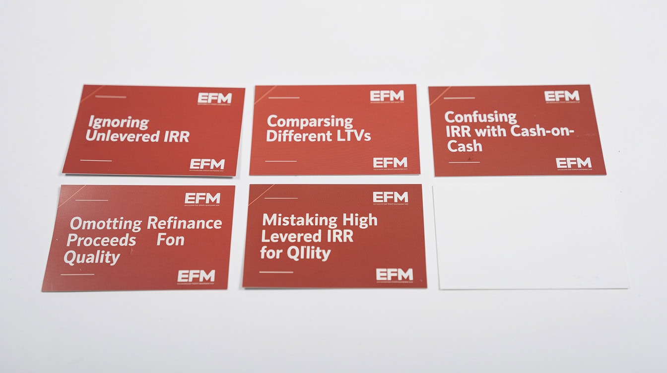
Each of these five pitfalls has caused real capital allocation errors — the most dangerous being the assumption that a 30% levered IRR automatically signals a high-quality deal.
Frequently Asked Questions
What is the difference between levered and unlevered IRR?
Unlevered IRR measures the return generated by an asset using only its operating cash flows, with no debt in the capital structure. It is also called the Project IRR. Levered IRR measures the return to equity holders after subtracting debt service (interest and principal repayment) from those same cash flows. The gap between the two reflects the impact of financial leverage. When debt costs 4% and the asset earns 7%, the 3-percentage-point spread accrues to equity, pushing levered IRR above unlevered IRR. The wider the spread and the higher the LTV, the larger the gap between the two metrics.
When is levered IRR higher than unlevered IRR?
Levered IRR exceeds unlevered IRR whenever the cost of debt is lower than the unlevered IRR. In the worked example above, a 7% unlevered return funded with 4% debt at 60% LTV produces a 12% levered IRR, according to BubbleGumBI. The positive spread of 3 percentage points between asset return and debt cost is the engine. If debt costs 9% on a 7% asset, the relationship reverses: levered IRR falls below unlevered IRR because each dollar of debt costs more than it earns, and equity absorbs the shortfall.
How do you calculate levered IRR in Excel?
Build a column of equity cash flows: enter the initial equity investment as a negative number in Year 0, then enter annual equity distributions (NOI minus debt service) for each year of the hold period, and add net sale proceeds (exit price minus remaining debt balance) in the final year. If a refinancing occurs mid-hold, add those proceeds as a positive cash flow in the relevant year. Then apply Excel’s =IRR() function to the entire cash flow range. Excel solves iteratively for the rate r that sets the NPV of that series to zero. For a full set of Excel formulas relevant to financial modeling, the 100 Excel Shortcuts and Formulas resource covers the IRR function and its variants in detail.
What is a good levered IRR for a real estate investment?
Target levered IRRs vary by strategy and risk profile. Core real estate (stabilized, low-risk assets) typically targets 8–12% levered IRR. Core-plus and value-add strategies target 12–18%. Opportunistic real estate and private equity buyouts typically require 20–30% or higher to compensate for execution risk. These ranges are not fixed benchmarks — they shift with interest rates, market conditions, and the specific asset class. The more important test is whether the unlevered IRR exceeds WACC, which confirms the asset creates value independently of financing.
Why does unlevered IRR stay the same when the capital structure changes?
Unlevered IRR is calculated from operating cash flows before any financing costs, so it reflects only the asset’s ability to generate returns from its business operations. Changing the debt-to-equity ratio does not alter NOI, CAPEX, depreciation, or working capital movements — the inputs to unlevered free cash flow. This is precisely why unlevered IRR is the correct metric for comparing assets with different capital structures: it isolates operating performance from financing decisions. Levered IRR, by contrast, changes every time the LTV, interest rate, or amortization schedule changes, even if the underlying asset is identical.
How does a mid-hold refinancing affect levered IRR?
A cash-out refinancing during the hold period returns capital to equity holders before the exit, which accelerates the timing of cash inflows. Because IRR weights earlier cash flows more heavily than later ones (due to the time value of money — the principle that a dollar today is worth more than a dollar in the future), receiving a large refinancing distribution in Year 3 of a 7-year hold can meaningfully boost levered IRR compared to receiving the same total proceeds only at exit. Analysts must include refinancing proceeds as a positive equity cash flow in the year received. Omitting them understates the true equity return and misrepresents the investment’s performance.
What is the relationship between levered IRR and the beta formula?
Both concepts separate the effect of financial leverage from underlying asset performance. The beta unlevering formula — βlevered = βunlevered × (1 + (1 − T) × D/E) — strips out the risk amplification caused by debt, just as unlevered IRR strips out the return amplification caused by debt. In a typical comparable company analysis, levered beta spans 1.10 to 1.55, while unlevered beta falls to 0.96 to 1.05, according to IB Interview Questions. The same compression logic applies to IRR: a 30% levered IRR at 90% LTV can correspond to a 7.7% unlevered IRR once the financing effect is removed. Both frameworks reveal that leverage is a magnifier, not a creator, of value.
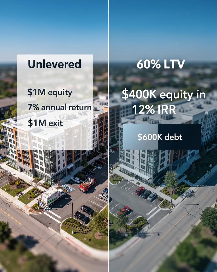
Experienced analysts run levered and unlevered IRR in parallel — one screen for asset quality, one for equity return — before committing capital.
Conclusion
Levered and unlevered IRR are not competing metrics — they are complementary lenses on the same investment. Unlevered IRR tells you whether the asset is worth owning. Levered IRR tells you whether the financing structure meets your equity return target. Use unlevered IRR to screen deals and compare assets on equal footing. Use levered IRR to size your debt and confirm your equity hurdle. Always verify that unlevered IRR exceeds WACC before relying on leverage to close the gap.
I recommend downloading the IRR modeling with multiple projects template to model your own levered and unlevered IRR scenarios side by side, with built-in sensitivity tables for LTV, debt cost, and exit valuation.