0 ITEMS

How to Build a Loan Amortization Table in Excel
To build a loan amortization table in Excel, put your loan inputs in labeled cells, calculate the fixed payment with the PMT function, then use IPMT and PPMT to split every payment into its interest and principal parts across an eight-column schedule. For a $100,000 loan at 5% over 15 years, =ROUND(PMT(B3/B5, B4*B5, -B2), 2) returns $790.79 per month, and every row of the table flows from that one figure. This guide walks through the whole build: the input layout, the PMT, IPMT and PPMT formulas, cumulative totals, rounding control, and the validation checks that prove the schedule closes to zero. Every number below comes from the same worked example, so you can follow it cell by cell.
Key Takeaways
- The PMT function calculates a fixed monthly payment in one cell: for a $100,000 loan at 5% over 15 years, the formula
=PMT(B3/B5, B4*B5, -B2)returns $790.79 per month. - A professional amortization table uses 8 columns: Period, Beginning Balance, Payment, Principal, Interest, Cumulative Principal, Cumulative Interest, and Ending Balance.
- Dividing the annual rate by 12 converts it to a monthly periodic rate — skipping this step overstates every interest charge by a factor of 12.
- Wrap every PMT result in
=ROUND(..., 2)to prevent penny-level rounding errors that leave a non-zero final balance. - IPMT and PPMT split each payment into its interest and principal components automatically, so you never need to calculate them by hand.
- Validate your finished schedule by confirming the Ending Balance in the final row equals zero (or within $0.01 due to rounding).
Understanding Loan Amortization Fundamentals
Amortization is the process of paying off a debt through scheduled, equal payments over time, where each payment covers both interest and a portion of the original loan balance (called the principal). An amortization schedule is a complete table showing exactly how much of each payment goes toward interest versus principal, and what the remaining balance is after every payment.
Businesses use amortization schedules to model debt service on equipment loans, commercial mortgages, and lines of credit. Individual borrowers use them to compare loan offers, plan early payoffs, and understand the true cost of borrowing. Without a schedule, it’s impossible to see that the first payment on a 30-year mortgage is mostly interest — and that the balance barely moves for years.
Three terms appear throughout this tutorial:
- Principal: The original amount borrowed (or the remaining unpaid balance at any point).
- Interest: The cost of borrowing, calculated as a percentage of the outstanding principal.
- Periodic rate: The annual interest rate divided by the number of payment periods per year (12 for monthly payments).
Setting Up Your Excel Input Variables
Before writing a single formula, place your loan parameters in clearly labeled input cells. This separation of inputs from calculations makes the model easy to audit and update.
Use this layout in your worksheet:
| Cell | Label | Value |
|---|---|---|
| A1 | Loan Amount | |
| B1 | 100000 | |
| A2 | Annual Interest Rate | |
| B2 | 5% | |
| A3 | Loan Term (Years) | |
| B3 | 15 | |
| A4 | Payments Per Year | |
| B4 | 12 | |
| A5 | Monthly Payment | |
| B5 | (formula goes here) |
For the worked example in this tutorial, inputs are mapped as B2 = $100,000 principal, B3 = 5% annual rate, B4 = 15 years, B5 = 12 payments per year, and B6 = the calculated monthly payment, the same B2:B6 input block used in MyExcelOnline’s guide to the amortization formula in Excel. Keep these references consistent throughout every formula below.
Absolute vs. relative cell references: An absolute reference (written with dollar signs, like $B$2) always points to the same cell regardless of where you copy the formula. A relative reference (like B2) shifts when you copy the formula down or across. In an amortization table, input cells like the interest rate and loan term must use absolute references so they don’t drift when you fill formulas down 360 rows.
Calculating the Fixed Monthly Payment with PMT
The PMT function (short for Payment) returns the fixed periodic payment required to fully repay a loan at a constant interest rate. Microsoft’s PMT function reference gives the syntax as =PMT(rate, nper, pv, [fv], [type]) — five arguments in total, the last two optional — where rate is the periodic interest rate, nper is the total number of payments, and pv is the present value (loan amount).
For the $100,000 example, enter this formula in cell B6:
=ROUND(PMT(B3/B5, B4*B5, -B2), 2)Here’s what each argument does:
- B3/B5 divides the 5% annual rate by 12 to get the monthly periodic rate of 0.4167%. You must divide by 12 because interest accrues monthly, not annually.
- B4*B5 multiplies 15 years by 12 payments per year to get 180 total payment periods.
- -B2 enters the loan amount as a negative number. PMT treats cash outflows as negative and inflows as positive. The loan principal is money you receive today (positive), so the payment it generates is an outflow (negative). Entering
-B2makes the returned payment a positive number, which is easier to read in a schedule. - ROUND(…, 2) rounds the result to 2 decimal places. Without rounding, floating-point arithmetic can leave a residual balance of a few cents at the end of the loan.
Result: =ROUND(PMT(5%/12, 15*12, -100000), 2) returns $790.79 per month, built with the same PMT construction shown in MyExcelOnline’s amortization formula walkthrough.
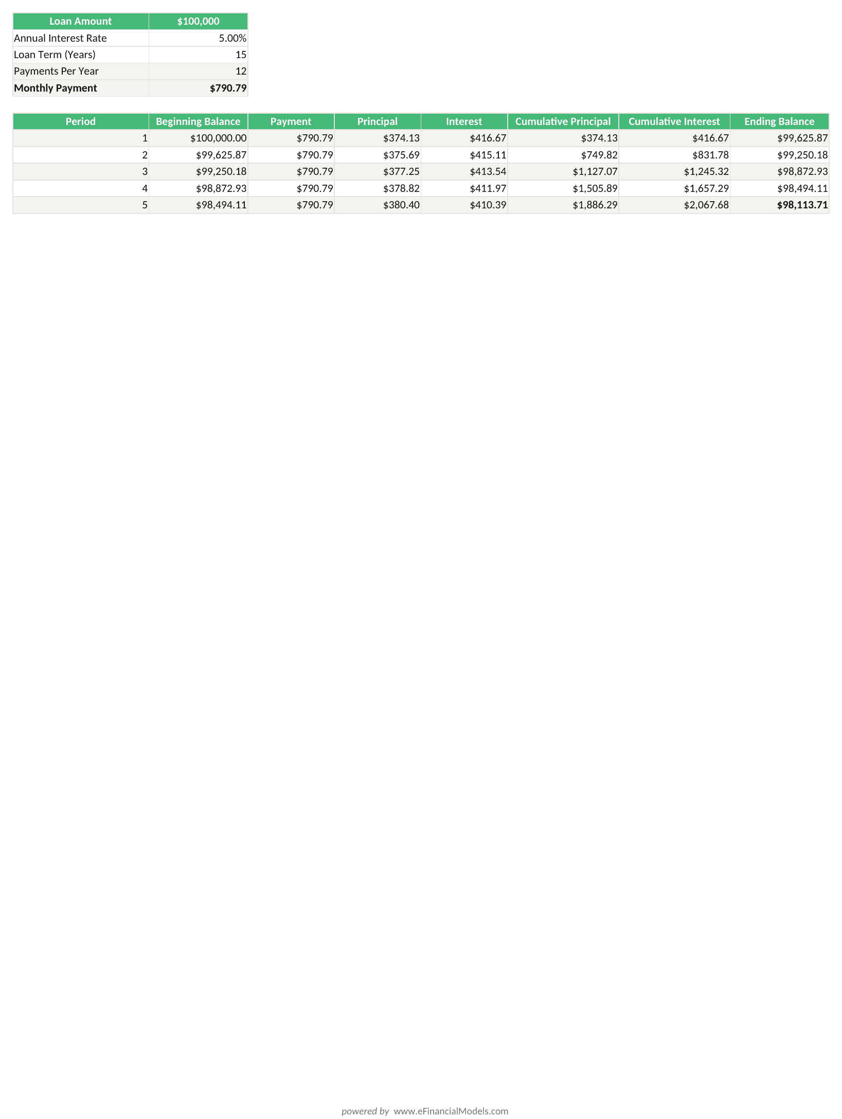
Monthly payment = $790.79 via =ROUND(PMT(B3/B5,B4*B5,-B2),2). Period 1 interest = $416.67; principal = $374.12; ending balance = $99,625.88.
Building the Eight-Column Amortization Table Structure
A professional amortization table uses 8 labeled columns that together show the full life of the loan. Place headers in row 7, with data starting in row 8.
Indeed’s eight-step guide to making an amortization schedule in Excel uses the same eight labels in row 7: Period (A7), Beginning Balance (B7), Payment (C7), Principal (D7), Interest (E7), Cumulative Principal (F7), Cumulative Interest (G7), and Ending Balance (H7).
Here is what each column tracks:
| Column | Header | Purpose |
|---|---|---|
| A | Period | Payment number (1, 2, 3 … 180) |
| B | Beginning Balance | Loan balance at the start of each period |
| C | Payment | Fixed monthly payment (same every row) |
| D | Principal | Portion of payment reducing the balance |
| E | Interest | Portion of payment covering interest charges |
| F | Cumulative Principal | Running total of all principal paid to date |
| G | Cumulative Interest | Running total of all interest paid to date |
| H | Ending Balance | Loan balance after this period’s payment |
Populating Payment Periods for Your Loan Term
Column A holds the period numbers that drive every other formula in the table. You have two efficient methods.
Method 1: Manual fill series. Type 1 in A8 and 2 in A9, select both cells, then drag the fill handle down. For a 30-year loan, fill down to row 367 — 360 monthly periods plus the 7 header rows above — which is the same range Indeed’s amortization schedule walkthrough fills for a 30-year term. For the 15-year example here, fill to row 187 (180 periods).
Method 2: SEQUENCE function (Excel 365/2019+). In cell A8, enter:
=SEQUENCE(B4*B5)For a 20-year loan, B4*B5 equals 20*12 = 240, so =SEQUENCE(240) spills all 240 period numbers automatically into column A. Microsoft’s SEQUENCE function reference documents its four arguments — rows, columns, start, and step — and confirms it returns a spilled array, which is what makes it ideal for auto-populating a period column without manual dragging. For a full video build of a loan schedule in Excel, see TrumpExcel’s Creating Loan Amortization Schedule in Excel (with Extra Payments).
Creating Formulas for Interest and Principal (IPMT and PPMT)
IPMT and PPMT are Excel’s built-in functions for splitting each payment into its interest and principal components. You don’t need to calculate these manually.
Interest for period 1 (cell E8):
=ROUND(IPMT($B$3/$B$5, A8, $B$4*$B$5, -$B$2), 2)$B$3/$B$5: periodic rate (absolute reference — must not shift when copied down)A8: the current period number (relative reference — shifts to A9, A10, etc. as you fill down)$B$4*$B$5: total number of periods (absolute)-$B$2: loan amount as negative (absolute)
For period 1 of the $100,000 loan: IPMT returns $416.67 (= $100,000 × 0.4167%).
Principal for period 1 (cell D8):
=ROUND(PPMT($B$3/$B$5, A8, $B$4*$B$5, -$B$2), 2)For period 1: PPMT returns $374.12 (= $790.79 payment minus $416.67 interest).
The same IPMT and PPMT pattern — a periodic rate of B3/B5 and total periods of B4*B5, copied down one row per payment — is set out in MyExcelOnline’s step-by-step amortization table instructions. Copy both formulas from row 8 down through the final period row.
Beginning Balance, Ending Balance, and Period-by-Period Changes
The Beginning Balance and Ending Balance columns create the cascading reduction of principal that defines amortization.
Beginning Balance (B8) — Period 1:
=B2The first period always starts with the full loan amount. For period 2 onward (B9 and below):
=H8This references the previous row’s Ending Balance, so each period’s Ending Balance becomes the next period’s Beginning Balance. Copy this formula down through all remaining periods.
Payment (C8):
=$B$6Absolute reference to the monthly payment cell. Every row returns the same fixed amount.
Ending Balance (H8):
=B8 - D8Ending Balance equals Beginning Balance minus the Principal portion of this period’s payment. Interest does not reduce the balance — it is the cost of carrying the balance. Copy this formula down through all periods.
Here’s the math for period 1:
- Beginning Balance: $100,000.00
- Payment: $790.79
- Interest (E8): $416.67
- Principal (D8): $374.12
- Ending Balance: $100,000.00 – $374.12 = $99,625.88
Tracking Cumulative Principal and Interest
Cumulative columns let you see the total cost of the loan at any point in time — useful for refinancing decisions and early payoff analysis.
Cumulative Principal (F8):
=SUM($D$8:D8)The first reference is absolute ($D$8) and the second is relative (D8). As you copy this formula down, the range expands: F9 sums D8:D9, F10 sums D8:D10, and so on. This is called an expanding range reference.
Cumulative Interest (G8):
=SUM($E$8:E8)Same expanding range logic applied to the Interest column.
By period 180 (the final payment on the 15-year loan), Cumulative Interest reaches approximately $42,342 — meaning the borrower pays $42,342 in interest on a $100,000 loan at 5% over 15 years. That figure alone justifies building this schedule before signing any loan agreement.
Rounding and Precision: Ensuring Your Final Balance Reaches Zero
Rounding errors are the most common reason a finished amortization schedule shows a small non-zero ending balance. Two practices prevent this.
First, wrap every PMT, IPMT, and PPMT call in =ROUND(..., 2). Microsoft’s ROUND function reference defines both of its arguments — the number and the digit count — as required, which makes the pattern easy to apply consistently across every payment component formula. Indeed’s amortization schedule guide applies exactly this pattern to the monthly payment, writing it as =ROUND(PMT($B$2/12,$B$3,-$B$1,0), 2).
Second, adjust the final period’s payment to absorb any residual. In the last row, replace the fixed payment formula with:
=B_last + E_lastWhere B_last is the final Beginning Balance and E_last is the final period’s interest. This forces the Ending Balance to exactly zero.
Comparison: Rounding Methods
| Method | Final Balance Error | Complexity | Recommended? |
|---|---|---|---|
| No rounding | Up to $2.00 residual | Low | No |
| ROUND on PMT only | Up to $0.10 residual | Low | Partial |
| ROUND on PMT + IPMT + PPMT | $0.00 to $0.01 | Medium | Yes |
| ROUND + final payment adjustment | Exactly $0.00 | Medium | Best practice |
Validating Your Schedule and Troubleshooting Common Errors
A correctly built amortization schedule passes three validation checks. Run these before using the model for any real decision.
- Validation check 1: The Ending Balance in the final row equals $0.00 (or within $0.01).
- Validation check 2: Cumulative Principal in the final row equals the original loan amount ($100,000).
- Validation check 3: Total payments (Payment × number of periods) equals Cumulative Principal + Cumulative Interest. For this example: $790.79 × 180 = $142,342.20, which should equal $100,000 + $42,342.20.
Common errors and fixes:
| Error | Cause | Fix |
|---|---|---|
#NUM! in PMT | Rate or nper is zero or negative | Check B3 and B4 are positive numbers |
#VALUE! in IPMT/PPMT | Period number (A8) is text, not a number | Reformat column A as Number |
| Circular reference warning | Ending Balance formula references itself | Ensure H8 = B8 – D8, not H8 – anything |
| Final balance not zero | Missing ROUND on IPMT/PPMT | Wrap all payment component formulas in ROUND |
| Balance goes negative | Period numbers exceed total nper | Confirm fill range matches B4*B5 exactly |
Adapting for different payment frequencies:
To switch from monthly to quarterly payments, change B5 from 12 to 4. All formulas referencing B5 update automatically because they use cell references, not hardcoded numbers. For biweekly payments, set B5 to 26. The periodic rate (B3/B5) and total periods (B4*B5) recalculate throughout the entire table without any other changes.
When to use this manual approach vs. Excel’s built-in templates: Excel’s built-in loan amortization template (available via File > New > search “loan amortization”) works for simple scenarios. Build your own when you need custom columns, scenario toggles, or integration with a larger financial model.
Frequently Asked Questions
Why does the PMT function require a negative loan amount?
Excel’s financial functions follow the cash flow sign convention: money you receive is positive, money you pay out is negative. When you take a loan, you receive the principal today (positive inflow), so the function expects pv to be positive. If you enter the loan amount as positive without the negative sign, PMT returns a negative payment, which works mathematically but looks confusing in a schedule. Entering -B2 (or -100000) makes the returned monthly payment a positive number, so your table reads naturally from top to bottom. This convention applies to all Excel financial functions including FV, PV, NPER, and RATE.
What is the difference between IPMT and PPMT, and do I need both?
IPMT calculates the interest portion of a specific payment, and PPMT calculates the principal portion. Together they always sum to the total payment: IPMT + PPMT = PMT. You technically need only one of them — if you know the total payment and the interest portion, the principal is the difference. However, using both functions explicitly and then verifying that D8 + E8 = C8 gives you a built-in accuracy check. For period 1 of the $100,000 example: IPMT = $416.67, PPMT = $374.12, total = $790.79. Any discrepancy signals a formula error.
How do I modify the schedule for a biweekly mortgage payment?
Change the Payments Per Year cell (B5) from 12 to 26. Every formula in the table references B5 for the periodic rate and total periods, so the entire schedule recalculates automatically. For a $100,000 loan at 5% over 15 years with biweekly payments, the total number of periods becomes 15 × 26 = 390. The periodic rate becomes 5% / 26 = 0.1923% per period. Biweekly payments result in 26 payments per year instead of 24 (twice monthly), which means you make the equivalent of one extra monthly payment per year and pay off the loan slightly faster.
Why does my final ending balance show $0.02 instead of $0.00?
This is a rounding accumulation error. Each period’s IPMT and PPMT values are rounded to 2 decimal places, and those small rounding differences accumulate over 180 or 360 periods. The fix is to wrap both IPMT and PPMT in =ROUND(..., 2) if you haven’t already, and then adjust the final period’s payment to exactly clear the remaining balance. In the last row, replace =$B$6 in the Payment column with =B_last + E_last (Beginning Balance plus final interest). This forces the Ending Balance to exactly $0.00 and is standard practice in professional loan models.
Can I use this template to compare two loan offers side by side?
Yes. The cleanest approach is to build two identical amortization tables on separate sheets, then create a summary sheet that pulls the key outputs: monthly payment, total interest paid, and payoff date. For example, comparing a $100,000 loan at 5% over 15 years ($790.79/month, $42,342 total interest) against the same loan at 4.5% over 20 years ($632.65/month, $51,836 total interest) shows that the longer term saves $158/month but costs $9,494 more in total interest. That trade-off is invisible without a schedule.
What does a #NUM! error mean in my amortization formula?
A #NUM! error in PMT, IPMT, or PPMT almost always means one of the numeric arguments is invalid. The most common causes are: the interest rate cell (B3) contains zero or a text value like “5%” formatted as text rather than a true percentage; the term cell (B4) is zero; or the payments-per-year cell (B5) is zero, which would create a division-by-zero in the rate argument. Check each input cell by selecting it and looking at the formula bar. If the value shows left-aligned, it’s stored as text. Reformat the cell as Number or Percentage and re-enter the value.
How do I make the schedule dynamic so it adjusts automatically when I change the loan term?
Use Excel Tables (Insert > Table) for the amortization rows, and combine them with the SEQUENCE function in column A. When you change B4 (years), update the SEQUENCE formula to =SEQUENCE(B4*B5) and the table expands or contracts automatically. For older Excel versions without dynamic arrays, use a helper column with =IF(A8<=$B$4*$B$5, A8, "") to suppress rows beyond the loan term. Named ranges (Formulas > Define Name) for inputs like LoanAmount, AnnualRate, and LoanTerm make formulas more readable and reduce errors when the model is shared with colleagues.
Build Your Amortization Model the Right Way
A well-built amortization table in Excel takes about 30 minutes to construct from scratch using the steps above. The PMT function handles the fixed payment, IPMT and PPMT split each payment into its components, and expanding SUM ranges track cumulative totals. The final validation check — confirming the ending balance reaches zero — tells you immediately whether every formula is correct.
For capital-intensive asset financing, you can pair this schedule with a broader debt structuring model. EFM’s mining industry financial model templates and stock market financial model templates both incorporate amortization logic. If you need a goodwill or impairment analysis alongside your debt schedule, the Goodwill Valuation and Impairment Test Model integrates cleanly with the approach shown here.
I recommend downloading EFM’s professional-grade Excel amortization template, which includes pre-built PMT, IPMT, and PPMT formulas, input validation, automatic period generation via SEQUENCE, and a scenario comparison panel for up to three loan offers side by side. It saves the setup time and eliminates the most common formula errors before you start.