CRE Acquisition Model Excel: Build It in 8 Steps

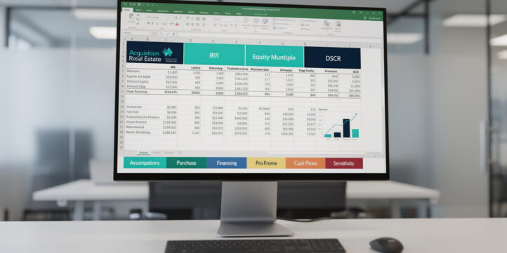
A commercial real estate acquisition model in Excel is the single analytical tool that determines whether a deal gets funded or killed — and building one correctly requires a specific worksheet architecture, formula logic, and return calculation sequence that most generic financial modeling guides skip entirely.

Key Takeaways

• A CRE acquisition model needs at least 6 linked worksheets: Assumptions, Purchase, Financing, Operating Pro Forma, Cash Flows, and Returns.
• Institutional investors typically target a levered IRR of 12-18% for value-add multifamily and 8-12% for stabilized core office, according to NCREIF benchmarks.
• Commercial lenders generally require a minimum debt service coverage ratio (DSCR) of 1.20x-1.25x, meaning net operating income must exceed annual debt service by at least 20-25%.
• Cap rates for Class A multifamily in primary markets averaged 4.5-5.5% in 2023, while industrial assets traded at 4.0-5.0%, per CBRE research.
• A 5-year hold with a Year 5 exit cap rate 50 basis points above the going-in cap rate is the most common base-case assumption in institutional underwriting.
• Sensitivity tables testing purchase price and exit cap rate simultaneously are the single most-requested output by investment committees.
• Pre-built Excel templates from eFinancialModels cut model build time from 40+ hours to under 4 hours for a standard acquisition.

What Is a Commercial Real Estate Acquisition Model?

A commercial real estate acquisition model is a structured Excel workbook that projects the cash flows, financing costs, and investment returns for a property purchase over a defined holding period, typically 5 to 10 years. It answers three questions for every deal: What does it cost to buy and operate? What does it return to equity investors? And how sensitive are those returns to changes in key assumptions?

This model differs from a development pro forma, which tracks construction draws and lease-up risk, and from a refinancing analysis, which focuses on debt restructuring. The acquisition model starts at closing and ends at disposition, capturing everything in between: rent growth, vacancy, capital expenditures, debt service, and the terminal sale.

Institutional buyers, private equity sponsors, family offices, and individual investors all use acquisition models. The structure is consistent across buyer types; the complexity scales with deal size and capital stack.

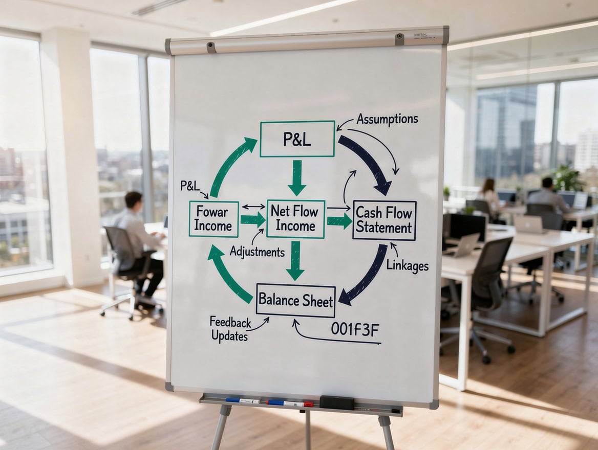
The 6-module chain ensures every output traces back to a single assumption input, eliminating hardcoded errors.

Essential Components of a CRE Acquisition Model in Excel

Every CRE acquisition model in Excel contains six core modules, each feeding the next in a logical chain. Skipping or combining modules creates circular reference errors (where a formula refers back to itself, causing Excel to loop endlessly) and makes auditing nearly impossible. Excel’s IRR function can handle an array of up to 29 cash flow values in its basic form (Source), which is more than sufficient for a standard 5- to 10-year hold period model.

The six modules are:

1. Purchase Price and Closing Costs — total acquisition basis including broker fees, transfer taxes, title insurance, and legal costs. Closing costs typically run 1-3% of purchase price for commercial transactions.
2. Financing Structure — loan amount, interest rate, amortization schedule, interest-only period, and balloon payment at exit.
3. Operating Pro Forma — gross potential rent, vacancy and credit loss, effective gross income, operating expenses, and net operating income (NOI). NOI is the property’s income before debt service and capital expenditures.
4. Capital Expenditure Reserve — tenant improvement allowances (TI), leasing commissions (LC), and capital reserves modeled as separate line items, not buried in operating expenses.
5. Cash Flow Waterfall — NOI minus debt service minus capex equals levered free cash flow distributed to equity investors.
6. Return Metrics — IRR (internal rate of return, the annualized return that makes the net present value of all cash flows equal zero), equity multiple, and cash-on-cash return for each year.

Excel Worksheet Structure and Architecture

The most efficient CRE acquisition model architecture uses one worksheet per module, with a dedicated Assumptions tab as the single source of truth. Every input lives on the Assumptions tab; every other tab pulls from it using direct cell references.

Here is the recommended tab order and purpose:

Use absolute cell references (locking a cell address with $ signs so it does not shift when copied, e.g., =$B$5) when pulling from the Assumptions tab. Use relative references (which shift automatically when copied) only within the same tab for row-by-row calculations like monthly amortization.

Name your key assumption cells using Excel’s Name Manager (Formulas tab, Define Name). Naming B5 as PurchasePrice makes formulas like =PurchasePrice*0.65 readable and auditable without hunting across tabs. A single Excel workbook can contain up to 255 sheets (Source), so there is no practical constraint on adding property-type-specific tabs as your model library grows.

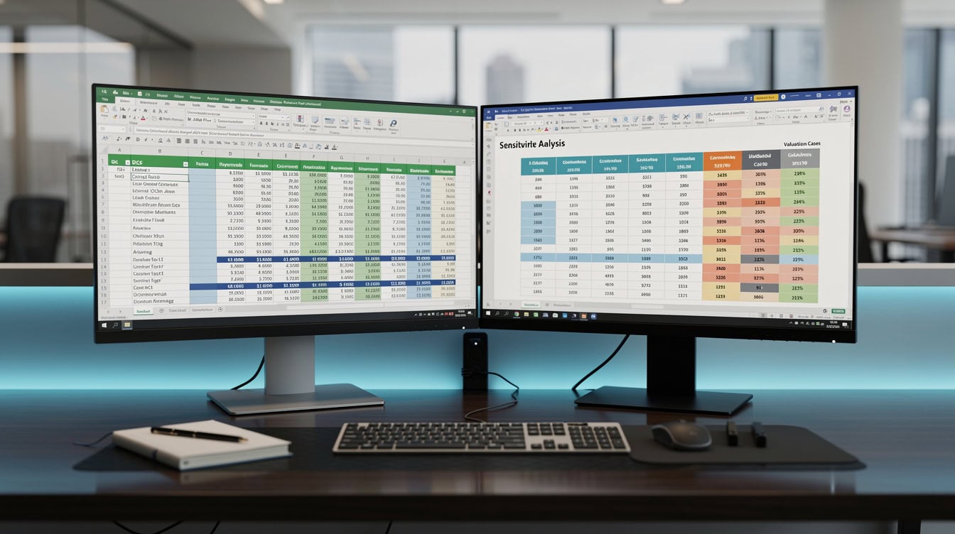
Named cells in the Assumptions tab (e.g., PurchasePrice, ExitCapRate) make formulas readable and auditable across all linked tabs.

Building the Purchase Price and Closing Costs Module

The Purchase tab calculates total acquisition basis, which is the all-in cost the model uses to size equity and compute returns. Start with the contract purchase price, then add each closing cost as a separate line item with its own percentage assumption on the Assumptions tab.

Worked Example: $10M Office Acquisition

Here’s the math for a $10,000,000 office building purchase:

• Purchase Price: $10,000,000
• Broker Fee (1.0%): $100,000
• Transfer Tax (0.5%): $50,000
• Title and Legal (0.3%): $30,000
• Loan Origination Fee (1.0% of loan): $65,000 (on a $6.5M loan)
• Immediate Capex Reserve: $200,000
• Total Acquisition Basis: $10,445,000

With a 65% loan-to-value (LTV) ratio, the loan is $6,500,000 and required equity is $3,945,000. The going-in cap rate equals Year 1 NOI divided by purchase price. If Year 1 NOI is $600,000, the going-in cap rate is 6.0% ($600,000 / $10,000,000).

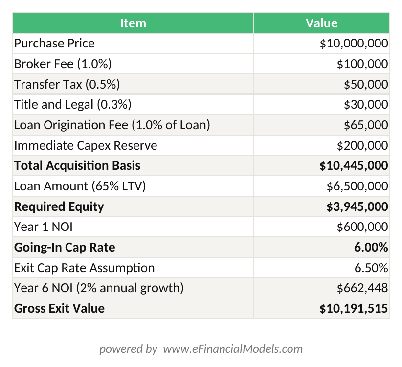
Going-in cap rate = Year 1 NOI / Purchase Price = 6.0%; Exit value at 6.5% cap on Year 6 NOI = $9.54M; Levered IRR ≈ 14.2%

The exit value in Year 5 uses an exit cap rate applied to Year 6 NOI (the buyer’s first year of ownership): =Year6_NOI / ExitCapRate. Selling costs of 1.5-2.0% reduce net sale proceeds before computing equity reversion.

Closing costs of 1-3% of purchase price add $180,000-$445,000 to the acquisition basis on a $10M deal, directly reducing equity returns.

Modeling Debt Financing and Loan Schedules in Excel

The Financing tab builds the full debt schedule, including interest-only periods, amortizing payments, and the balloon payment due at exit. Commercial lenders generally require a minimum DSCR of 1.20x-1.25x (Source), meaning NOI must cover annual debt service by at least that margin.

For a $6,500,000 loan at 6.5% interest, 25-year amortization, with a 2-year interest-only period:

• Years 1-2 (Interest Only): Annual interest = $6,500,000 × 6.5% = $422,500
• Years 3-10 (Amortizing): Use Excel’s =PMT(rate/12, nper, pv) function to calculate monthly payment, then multiply by 12 for annual debt service. The PMT function accepts up to 5 arguments (Source) and is the standard tool for fixed-payment loan schedules in CRE models.
• =PMT(6.5%/12, 25*12, -6500000) = approximately $43,900/month = $526,800/year
• Year 5 Balloon: Use =FV(rate/12, periods, payment, pv) to calculate the outstanding balance at the end of Year 5, which becomes the balloon payment due at sale.

For bridge loans (short-term floating-rate loans used for value-add acquisitions before stabilization), model the interest rate as a spread over SOFR (the Secured Overnight Financing Rate, which replaced LIBOR as the benchmark for floating-rate debt). Build a SOFR assumption on the Assumptions tab so you can stress-test rising rate scenarios.

Mezzanine debt (a second layer of financing that sits between senior debt and equity, typically at 10-14% interest) adds a second loan block to the Financing tab. Model it identically to senior debt but with its own rate, term, and repayment priority in the waterfall.

A 2-year interest-only period reduces early debt service by $104,300/year on a $6.5M loan, improving initial DSCR and cash-on-cash returns.

Constructing the Operating Pro Forma

The Pro Forma tab projects revenue and expenses for each year of the holding period. Build it in this sequence: gross potential rent, then vacancy and credit loss, then other income, then operating expenses, then NOI.

Revenue section:

• Gross Potential Rent (GPR): Current in-place rent escalated by an annual rent growth assumption (typically 2-4% for multifamily, 1-3% for office)
• Vacancy and Credit Loss: GPR multiplied by a vacancy rate assumption. CBRE data shows stabilized multifamily vacancy averaged 5.8% nationally in 2023, while office vacancy in major markets exceeded 18%.
• Other Income: Parking, laundry, storage, or ancillary fees
• Effective Gross Income (EGI): GPR minus vacancy plus other income

Expense section:
Operating expense ratios (total operating expenses as a percentage of EGI) vary significantly by property type. According to the Institute of Real Estate Management (IREM), typical expense ratios run 35-45% for multifamily, 40-55% for office (which carries higher management and maintenance costs), and 15-25% for net-lease industrial (where tenants pay most expenses directly).

Model each expense line separately: property taxes, insurance, management fee (typically 3-5% of EGI), maintenance and repairs, utilities, and administrative costs. Never lump them into a single percentage — lenders and investment committees will reject that level of imprecision.

Capital expenditures below the NOI line:

• Tenant Improvement Allowances: For office, budget $40-80 per square foot for new leases and $20-40 for renewals, per CBRE leasing cost data.
• Leasing Commissions: Typically 4-6% of total lease value for new leases, 2-3% for renewals.
• Capital Reserves: $250-350 per unit per year for multifamily; $0.15-0.25 per square foot per year for industrial.

Operating expense ratios range from 15-25% for NNN industrial to 40-55% for office, making property-type-specific line items essential.

Cash Flow Waterfall and Return Calculations

The Cash Flows tab assembles all prior tabs into a single timeline of cash flows, then the Returns tab computes investment performance metrics. The waterfall (the sequence in which cash flows are distributed to different capital providers) runs: NOI, then subtract debt service, then subtract capex, then distribute remaining cash to equity.

The three return metrics every investment committee requires:

1. IRR (Internal Rate of Return): Use =IRR(cash_flow_range) in Excel. The cash flow range starts with the initial equity investment as a negative number (cash out), followed by annual levered free cash flows, with the equity reversion added to the final year. A levered IRR of 15% on a value-add multifamily deal means equity investors earn 15% annually on their invested capital, accounting for the timing of all cash flows.

1. Equity Multiple (EM): Total cash returned to equity divided by total equity invested. =SUM(all_equity_distributions) / initial_equity. An equity multiple of 1.8x means investors receive $1.80 for every $1.00 invested. Institutional value-add targets typically require 1.7x-2.2x over a 5-year hold.

1. Cash-on-Cash Return (CoC): Annual levered free cash flow divided by initial equity invested. =Year_N_FCF / Initial_Equity. This metric matters most to income-focused investors who need current yield, not just terminal returns.

According to NCREIF (National Council of Real Estate Investment Fiduciaries), core real estate strategies historically target 8-10% total returns, while value-add strategies target 12-18% levered IRR (Source).

The waterfall sequence (NOI minus debt service minus capex) determines levered free cash flow, which drives IRR and equity multiple calculations.

Property Type-Specific Model Adjustments

The base model structure stays consistent across property types, but revenue drivers, expense line items, and lease structures differ materially. Applying a multifamily model to an office deal without adjustment will produce incorrect NOI and misleading returns.

For multifamily, model rent at the unit level (studio, 1BR, 2BR) with separate vacancy rates by unit type. For office, model each tenant’s lease separately with expiration dates, renewal probability, and downtime between leases. For retail, include a percentage rent clause (additional rent triggered when tenant sales exceed a breakpoint). For industrial, the model is simplest: NNN leases mean tenants pay taxes, insurance, and maintenance directly, so the landlord’s expense line is minimal.

Sensitivity Analysis and Scenario Testing

Sensitivity analysis in Excel uses Data Tables (a built-in Excel feature that recalculates a formula across a grid of input values) to show how IRR changes when two assumptions vary simultaneously. This is the most powerful output in any CRE acquisition model.

To build a two-variable data table for IRR vs. purchase price and exit cap rate:

1. Place the IRR formula in a cell (e.g., =IRR(C5:C15)) at the top-left corner of your table range.
2. List purchase price variations across the top row (e.g., $9M, $9.5M, $10M, $10.5M, $11M).
3. List exit cap rate variations down the left column (e.g., 5.0%, 5.5%, 6.0%, 6.5%, 7.0%).
4. Select the full table range, go to Data, What-If Analysis, Data Table, and assign the row input cell (purchase price assumption) and column input cell (exit cap rate assumption).
5. Excel populates every cell in the grid with the IRR at that combination of inputs.

Color-code the table using conditional formatting: green for IRR above your hurdle rate (e.g., 15%), yellow for 10-15%, red for below 10%. Investment committees read this table in seconds and immediately see the deal’s risk profile.

Build a separate Scenario Manager (Data, What-If Analysis, Scenario Manager) for named scenarios: Base Case, Bull Case (higher rent growth, lower exit cap), and Bear Case (higher vacancy, higher exit cap, rising rates). Each scenario stores a complete set of assumption values and lets you switch between them with one click.

Common Excel Errors in CRE Acquisition Models

Five mistakes appear repeatedly in CRE acquisition models built without a structured template:

1. Circular references in construction interest calculations. When interest accrues on a loan balance that itself includes prior interest, Excel creates a circular reference. Fix this by enabling iterative calculation (File, Options, Formulas, Enable Iterative Calculation) or by breaking the circularity with a prior-period balance reference.

2. Hardcoded numbers in formula cells. Typing =600000*1.03 instead of =NOI_Year1*(1+RentGrowth) makes the model impossible to audit and breaks when assumptions change. Every variable must trace back to the Assumptions tab.

3. Mixing pre-tax and after-tax cash flows. CRE acquisition models typically operate on a pre-tax basis for the operating cash flows, then apply depreciation and tax benefits separately. Mixing the two in the same cash flow column produces IRR figures that are neither pre-tax nor after-tax, and therefore meaningless.

4. Incorrect IRR formula range. The =IRR() function requires the initial equity investment as a negative number in the first cell of the range. Omitting the negative sign or starting the range in Year 1 instead of Year 0 produces a wildly incorrect IRR. Always verify: =IRR({-3945000, 150000, 175000, 200000, 225000, 4500000}) should return approximately 14.2% for this example.

5. Ignoring lease-up timing in the pro forma. Assuming 100% occupancy from Day 1 on a value-add acquisition overstates early-year NOI. Model a lease-up curve: 70% occupancy in Month 1, ramping to 93% by Month 18, with corresponding TI and LC costs in those early periods.

Pre-Built Templates vs. Custom Models

Building a CRE acquisition model from scratch takes an experienced analyst 30-50 hours for a fully functional, multi-property-type model. Pre-built templates from eFinancialModels deliver the same functionality in under 4 hours of customization, with pre-configured worksheets, dynamic sensitivity tables, and built-in error checks already in place.

Choose a pre-built template when: you need to evaluate a deal quickly, you lack a senior modeler to build from scratch, or you want a consistent format across multiple deals for portfolio comparison.

Build from scratch when: the deal has a highly unusual structure (ground lease, EB-5 financing, complex joint venture waterfall) that no template accommodates, or when your firm requires a proprietary model format for investment committee presentations.

When evaluating any pre-built template, verify these 5 must-have features:

1. Dynamic loan schedule with interest-only toggle
2. Two-variable sensitivity data tables (not just single-variable)
3. Separate capex module below the NOI line
4. Property-type selector that adjusts revenue and expense line items
5. Unlocked cells so you can customize assumptions without breaking formulas

EFM’s commercial real estate financial models include all five features and cover multifamily, office, retail, and industrial property types. For analysts who need a broader library of real estate valuation templates, EFM’s catalog includes DCF-based models, waterfall distribution models, and three-statement real estate models.

For teams that need a custom financial modeling service for a deal with a non-standard structure, EFM also offers bespoke model builds.

Frequently Asked Questions About CRE Acquisition Models in Excel

What is the standard holding period assumption in a CRE acquisition model?

The most common holding period in institutional CRE underwriting is 5 years, though value-add deals with longer lease-up timelines often use 7 years and core office or retail deals frequently model 10 years. The holding period directly affects IRR because longer holds dilute the impact of the equity reversion on the annualized return. A deal returning 1.8x equity multiple over 5 years produces a 12.5% IRR; the same 1.8x multiple over 10 years produces only a 6.1% IRR. Always model at least two holding periods (5-year and 7-year) in your sensitivity table to show the committee how time affects returns.

What DSCR do commercial lenders require for CRE acquisitions?

Most commercial lenders require a minimum debt service coverage ratio of 1.20x to 1.25x at origination, meaning the property’s NOI must exceed annual debt service by 20-25%. Agency lenders (Fannie Mae, Freddie Mac) for multifamily typically require 1.25x DSCR at a stressed interest rate (often 25-50 basis points above the actual note rate). Life insurance companies and CMBS lenders for office and retail often require 1.30x-1.40x given higher vacancy risk. Model your DSCR as =NOI / Annual_Debt_Service and flag any year where it falls below 1.20x with a conditional format alert.

How do I handle tenant improvement allowances and leasing commissions in the model?

Tenant improvement allowances (TI) and leasing commissions (LC) are capital expenditures that appear below the NOI line in the cash flow waterfall, not as operating expenses. Model them as lump-sum outflows in the year a lease commences or renews. For a 10,000 square foot office tenant signing a 5-year lease with a $50/SF TI allowance and a 5% leasing commission on $30/SF annual rent, the Year 1 capex is: TI = $500,000 plus LC = $75,000 (5% × $30 × 10,000 × 5 years) = $575,000 total. Spreading these costs incorrectly as annual operating expenses understates NOI and overstates DSCR, which will cause problems during lender underwriting review.

What is the difference between going-in cap rate and exit cap rate in an acquisition model?

The going-in cap rate is Year 1 NOI divided by the purchase price, representing the initial yield on the investment. The exit cap rate is the rate applied to the final year’s NOI (or the following year’s projected NOI) to calculate the sale price at the end of the holding period. Institutional underwriting convention applies the exit cap rate to the year after the last hold year: if you hold for 5 years, apply the exit cap to Year 6 NOI. The exit cap rate is almost always modeled 25-75 basis points above the going-in cap rate to reflect asset aging, market uncertainty, and the buyer’s required return premium. A 50 basis point expansion on a $600,000 NOI property reduces the exit value by approximately $1.7M on a 5.5% exit cap versus a 5.0% going-in cap.

How do I build a two-variable sensitivity table in Excel for IRR?

A two-variable data table in Excel (also called a two-way data table) recalculates a single output formula across a grid of two input variables. Place your IRR formula in the top-left corner of the table. Enter purchase price scenarios across the top row and exit cap rate scenarios down the left column. Select the entire table range including the corner formula and both input rows/columns. Go to Data, What-If Analysis, Data Table. In the Row Input Cell field, select the purchase price assumption cell on your Assumptions tab. In the Column Input Cell field, select the exit cap rate assumption cell. Click OK and Excel fills every cell in the grid. The result is a complete IRR matrix showing, for example, that at a $10M purchase price and 6.0% exit cap, IRR is 13.8%, while at $10.5M and 6.5% exit cap, IRR drops to 9.2%.

What return thresholds do institutional investors use for different CRE property types?

Return thresholds vary by strategy and property type. Core strategies (stabilized, low-risk assets in primary markets) target 7-9% unlevered IRR and 8-11% levered IRR. Value-add strategies (properties requiring repositioning or lease-up) target 12-16% levered IRR and a 1.7x-2.2x equity multiple. Opportunistic strategies (ground-up development or distressed assets) target 18-25%+ levered IRR. By property type, industrial and multifamily command lower return thresholds (tighter cap rates, more liquid markets) while office and retail require higher return premiums given elevated vacancy and leasing risk. According to NCREIF performance data, the 10-year average total return for core real estate was approximately 8.5% annually through 2023.

Can I use the same Excel acquisition model for a portfolio of multiple properties?

Yes, but the architecture changes. A single-asset model uses one Pro Forma tab; a portfolio model adds a Summary tab that aggregates NOI, debt service, and cash flows across all assets, with each property on its own tab following the same structure. The Returns tab then computes portfolio-level IRR using the combined equity investment and blended cash flows. EFM’s real estate financial models include multi-property templates with a master summary dashboard. For portfolio-level analysis, also build a correlation matrix showing how different assets’ cash flows offset each other during stress scenarios, which strengthens the investment committee presentation.

Conclusion

A well-built commercial real estate acquisition model in Excel is not a luxury for large institutional deals — it is the minimum standard for any serious CRE investment decision. The 8-step architecture outlined here (Assumptions, Purchase, Financing, Pro Forma, Cash Flows, Returns, Sensitivity, and Error Checks) gives you a model that survives lender scrutiny, investment committee review, and post-close performance tracking.

The difference between a model that gets a deal approved and one that kills it often comes down to three things: accurate capex modeling below the NOI line, a properly structured debt schedule with DSCR checks, and a two-variable sensitivity table that shows the committee exactly where the deal breaks.

I recommend downloading the eFinancialModels Commercial Real Estate Acquisition Model to get a professionally structured Excel workbook with all six tabs pre-configured, dynamic sensitivity tables, and property-type selectors built in — so you can focus on the deal, not the spreadsheet architecture.

by eFinancialModels

Solar Energy Financial Model

Average rating:

The Solar Energy Financial Model Spreadsheet Template in Excel assists you in preparing a sophisticated financial forecast for a utility-scale solar p... read more

•  PREMIUM – $149.95 Version 7.4
•  PRO – $129.95 Version 7.4
•  BASIC – $99.95 Version 7.4
•  PDF Demos – $0.00 Version 7.4

Add to wish list

Purchase Checkout Added to cart Excluding 0% tax

by eFinancialModels

Financial Model for Mobile App | Mobile App Business Plan

Average rating:

The Mobile App Financial Plan Template in Excel allows you to develop financial projections when launching a new business centered around an app insta... read more

•  PREMIUM – $209.95 Version 7.3
•  PRO – $159.95 Version 7.3
•  BASIC – $109.95 Version 7.3
•  PDF Demo Versions – $0.00 Version 7.3

Add to wish list

Purchase Checkout Added to cart Excluding 0% tax

by Street Fox Advisors

Private Equity Fund Model (Investor Cashflows)

Average rating:

The Private Equity Fund Cashflows Model helps LPs and GPs analyze fund cash flows, returns, and distributions across investor, manager, and portfolio ... read more

•  PDF Demo version – $0.00 Version 3
•  European Waterfall – $105.00 Version 3
•  American Waterfall – $125.00 Version 3

Add to wish list

Purchase Checkout Added to cart Excluding 0% tax

by eFinancialModels

Pharma Biotech Valuation Model Template (Risk-Adjusted)

Average rating:

The Pharma Biotech Valuation Model Template calculates the risk-adjusted DCF Value of a Pharma or Biotech Startup Company with several products under ... read more

•  Full Excel Model - PREMIUM – $199.95 Version 2.2
•  Full Excel Model - BASIC – $149.95 Version 2.2
•  PDF Demo Previews – $0.00 Version 2.2

Add to wish list

Purchase Checkout Added to cart Excluding 0% tax

by eFinancialModels

SaaS Business Financial Model

Average rating:

The SaaS Business financial model offers valuable assistance in preparing a budget and multi-year financial plan for a Software as a Service (SaaS) bu... read more

•  Premium Excel Model – $199.95 Version 8.2
•  Pro Excel Model – $149.95 Version 8.2
•  Basic Excel Model – $99.95 Version 8.2
•  PDF Demo – $0.00 Version 8.2

Add to wish list

Purchase Checkout Added to cart Excluding 0% tax

by FinModelsLab

Coffee Shop Financial Model Excel Template

Average rating:

The Coffee Shop Financial Model helps entrepreneurs, founders, business owners, consultants, and analysts turn a cafe concept into a structured financ... read more

•  Excel - Multi-User – $129.00 Version 1
•  Excel - Single-User – $99.00 Version 1

Add to wish list

Purchase Checkout Added to cart Excluding 0% tax

by eFinancialModels

Free Discounted Cash Flow (DCF) Valuation Model Template

Average rating:

This Discounted Cash Flow (DCF) valuation calculator template projects a three-statement model that allows users to value a company based on the net p... read more

•  Pro Version – $0.00 Version 4.5
•  Basic Version – $0.00 Version 4.5
•  Cup of Coffee – $5.00 Version 4.5

Add to wish list

Purchase Checkout Added to cart

by eFinancialModels

Hotel Investment Financial Model

Average rating:

The Hotel Investment Financial Model provides a framework to forecast the expected cash flows for a hotel investment and calculates the relevant inves... read more

•  FULL Version (Excel) – $34.95
•  FREE Version (PDF) – $0.00

Add to wish list

Purchase Checkout Added to cart Excluding 0% tax

by FinModelsLab

Hotel Financial Model Excel Template

Average rating:

The Hotel Financial Model helps users build a structured financial forecast for a hotel business using the revenue drivers that matter most in hospita... read more

•  Excel - Multi-User – $129.00 Version 1
•  Excel - Single-User – $99.00 Version 1

Add to wish list

Purchase Checkout Added to cart Excluding 0% tax

by eFinancialModels

Upstream Oil & Gas Project Analysis

Average rating:

The Upstream Oil & Gas Project Financial Model Template in Excel empowers you to project and dissect your impending Oil and Gas drilling ventures. Pre... read more

•  Pro - Full Excel Model – $159.95 Version 8.3
•  Basic - Full Excel Model – $119.95 Version 8.3
•  PDF Demo Versions – $0.00 Version 8.3

Add to wish list

Purchase Checkout Added to cart Excluding 0% tax

by smarthelping

All My Financial Models, Spreadsheets, Templates, and Tools: 120+

Average rating:

Lifetime access to all future templates as well! Here is a set of spreadsheets that have some of the most valuable logic in the world. I have been thr... read more

•  All My Excel Tools – $499.00 Version 1

Add to wish list

Purchase Checkout Added to cart Excluding 0% tax

by eFinancialModels

Google Sheets Project Plan Template

Average rating:

This Project Plan Template in Google Sheet allows you to quickly develop a project plan and plot a Gantt chart. Enjoy all the benefits of Google Docs ... read more

•  Free Excel Template – $0.00 Version 1
•  Cup of Coffee – $5.00 Version 1

Add to wish list

Purchase Checkout Added to cart Excluding 0% tax

by eFinancialModels

Commercial Real Estate Valuation Model Template

Average rating:

A commercial real estate valuation model template assists in running a professional DCF Valuation for a commercial property such as an office building... read more

•  PDF Demo Versions – $0.00 Version 1
•  BASIC Excel Model Template – $59.00 Version 1
•  PRO Excel Model Template – $99.00 Version 1
•  PREMIUM Excel MODEL + Report Template – $199.00 Version 1

Add to wish list

Purchase Checkout Added to cart Excluding 0% tax

by eFinancialModels

Waterfall Profit Distribution Model (up to 4 Tiers)

Average rating:

We are introducing our 4-Tier Waterfall Profit Distribution Model. The waterfall profit distribution model template aims to support a thorough analysi... read more

•  Full Excel Model – $79.95 Version 2.1
•  PDF Demo – $0.00 Version 2.1

Add to wish list

Purchase Checkout Added to cart Excluding 0% tax

by eFinancialModels

Wind Energy Farm Financial Model

Average rating:

The Wind Farm Financial Model provides a powerful 40-year forecast, capturing critical data on energy production, revenues, operating costs, and debt ... read more

•  Excel Version – $149.95 Version 4.2
•  PDF Version – $0.00 Version 4.2

Add to wish list

Purchase Checkout Added to cart Excluding 0% tax

by AM Financial Models

Private School Financial Model

Average rating:

This is a financial model template for a new private school startup business. The Excel model allows forecasting the cash flows over the next 10 years... read more

•  Excel Model – $44.95 Version 9.1
•  PDF Demo – $0.00 Version 9.0

Add to wish list

Purchase Checkout Added to cart Excluding 0% tax

by eFinancialModels

Free Three Statement Financial Model

Average rating:

Feeling overwhelmed by the daunting task of financial forecasting? This FREE Download 5-Year Three Statement Financial Model Excel Template offers you... read more

•  Free Excel Template – $0.00 Version 2.7
•  Cup of Coffee – $5.00 Version 2.7

Add to wish list

Purchase Checkout Added to cart Excluding 0% tax

by Profit Vision

Advanced Financial Model with DCF and Valuation

Average rating:

Dynamic 10-Year Financial Model, suitable for any type of business, supporting strategic planning, investment decisions, and business valuation.

•  Excel Financial Model – $139.00 Version 1
•  PDF Free Demo – $0.00 Version 1

Add to wish list

Purchase Checkout Added to cart Excluding 0% tax

by eFinancialModels

Green Hydrogen (Electrolysis) Production Financial Model

Average rating:

This green hydrogen financial model template builds a multi-year financial plan to analyze the financial feasibility and profitability for the product... read more

•  Full Excel Version – $119.00 Version 1.8
•  PDF Version – $0.00 Version 1.8

Add to wish list

Purchase Checkout Added to cart Excluding 0% tax

by eFinancialModels

Gasoline and EV Charging Station Financial Model

Average rating:

Investors can assess the viability of setting up and investing in gasoline stations with a charging station by downloading a financial model for their... read more

•  Premium Excel Version – $129.95 Version 2.1
•  Basic Excel Version – $99.95 Version 2.1
•  PDF Versions – $0.00 Version 2.1

Add to wish list

Purchase Checkout Added to cart Excluding 0% tax

by FinModelsLab

Grocery Store Financial Model Excel Template

Average rating:

The Grocery Store Financial Model helps entrepreneurs, founders, consultants, analysts, and retail business owners build a structured financial foreca... read more

•  Excel - Multi-User – $129.00 Version 1
•  Excel - Single-User – $99.00 Version 1

Add to wish list

Purchase Checkout Added to cart Excluding 0% tax

by eFinancialModels

Manufacturing Company Financial Model

Average rating:

The Manufacturing Financial Model provides a framework to accurately forecast the financial statements of a manufacturing company over the next 10 yea... read more

•  Excel Model – $44.95 Version 4
•  PDF Demo – $0.00 Version 4

Add to wish list

Purchase Checkout Added to cart Excluding 0% tax

by smarthelping

Fitness Center 10 Year Financial Model

Average rating:

Key logic designed to forecast cash flow up to 10 years for a fitness center that has recurring monthly fees. Fully integrated 3-statement model, cap ... read more

Add to wish list

$75.00 – Purchase Checkout Added to cart Excluding 0% tax

by Bassem Mneimne

Green Hydrogen (Simple Electrolysis Financial Model)

Average rating:

The Model Incorporates data provided by different available sources to Model an Electrolysis financial model. It includes Electrolyzer cost, Dispenser... read more

•  Excel Template – $150.00 Version 1
•  Free Version – $0.00 Version 1

Add to wish list

Purchase Checkout Added to cart Excluding 0% tax

by FinModelsLab

Outpatient Clinic Financial Model Excel Template

Average rating:

The Outpatient Clinic Financial Model helps users turn a clinic business concept into a structured, editable financial forecast. Instead of relying on... read more

•  Excel - Multi-User – $129.00 Version 1
•  Excel - Single-User – $99.00 Version 1

Add to wish list

Purchase Checkout Added to cart Excluding 0% tax

by Big4WallStreet

Airbnb Financial Model

Average rating:Submit Rating

Air BnB Financial Model Template presents the business case of the purchase of up to 5 properties with the intent of utilizing them as short term rent... read more

•  Excel Model – $119.00 Version 1
•  Free PDF – $0.00 Version 1

Add to wish list

Purchase Checkout Added to cart Excluding 0% tax

by smarthelping

Lending Platform Financial Model (LaaS)

Average rating:

Includes all the assumptions you need to project the gross revenues and profits of a LaaS platform (Lending as a Service). 3-statement model and cap t... read more

•  Excel Model – $75.00 Version 3

Add to wish list

Purchase Checkout Added to cart Excluding 0% tax

by eFinancialModels

Beverage Manufacturing Start-Up Financial Model

Average rating:

The beverage manufacturing industry is a dynamic and rapidly growing sector that caters to a diverse market ranging from soft drinks and juices to alc... read more

•  Excel Model – $249.95 Version 5.3
•  PDF Demo – $0.00 Version 5.3

Add to wish list

Purchase Checkout Added to cart Excluding 0% tax

by eFinancialModels

Simple Cap Table Template – Free Download

Average rating:

This is a simple capitalization (cap) table template which allows entrepreneurs to understand the dilution effect of capital raisings and a simple sto... read more

•  Free Excel Template – $0.00 Version 1
•  Cup of Coffee – $5.00 Version 1

Add to wish list

Purchase Checkout Added to cart Excluding 0% tax

by Profit Vision

Startup Company Financial Model – 5 Year Financial Forecast

Average rating:

Highly-sophisticated and user-friendly financial model for Startup Companies providing a 5-Year advanced financial forecast.

•  Financial Model - Light Version – $119.00 Version 1
•  Financial Model - Standard Version – $159.00 Version 1
•  Financial Model - Premium Version – $219.00 Version 1
•  PDF Free Demo – $0.00 Version 1

Add to wish list

Purchase Checkout Added to cart Excluding 0% tax

by eFinancialModels

Gold Mine Investment Model

Average rating:

The Gold Mine Investment Model is used to determine the financial feasibility of a proposed Gold Mine Investment. The Financial Model outputs IRR and ... read more

•  Excel Financial Model – $44.95 Version 6.2
•  PDF Demo – $0.00 Version 6.2

Add to wish list

Purchase Checkout Added to cart Excluding 0% tax

by FinModelsLab

Bakery Financial Model Excel Template

Average rating:

The Bakery Financial Model helps entrepreneurs, bakery owners, consultants, analysts, and business plan writers turn a bakery concept into a structure... read more

•  Excel - Multi-User – $129.00 Version 1
•  Excel - Single-User – $99.00 Version 1

Add to wish list

Purchase Checkout Added to cart Excluding 0% tax

by Big4WallStreet

Airport Operator Financial Model

Average rating:

Airport Operator Financial Model presents the business case of an already operating airport (with planned refurbishments) and an investment in a new t... read more

•  Excel Model – $119.00
•  Free PDF – $0.00

Add to wish list

Purchase Checkout Added to cart Excluding 0% tax

by FinModelsLab

Cafe Financial Model Excel Template

Average rating:

The Cafe Financial Model is a ready-to-use financial model template designed to help entrepreneurs, cafe owners, founders, consultants, and analysts b... read more

•  Excel - Multi-User – $129.00 Version 1
•  Excel - Single-User – $99.00 Version 1

Add to wish list

Purchase Checkout Added to cart Excluding 0% tax

by Pierre-Alexandre Heurtebize

Due Diligence P&L – Exhaustive Revenue and Costs Analysis Template

Average rating:Submit Rating

Model for in depth understanding of high level profit and loss and revenue analysis. Big-4 like checklist of due diligence analyses. This Financial Du... read more

Add to wish list

$250.00 – Purchase Checkout Added to cart Excluding 0% tax

by FinModelsLab

Clothing Store Financial Model Excel Template

Average rating:

The Clothing Store Financial Model helps turn a retail apparel concept into a structured financial forecast that can be used for planning, funding, bu... read more

•  Excel - Multi-User – $129.00 Version 1
•  Excel - Single-User – $99.00 Version 1

Add to wish list

Purchase Checkout Added to cart Excluding 0% tax

by FinModelsLab

Poultry Farm Financial Model Excel Template

Average rating:

The Poultry Farming Financial Model helps users turn a poultry farm concept into a structured, lender-ready financial forecast. It is designed for pla... read more

•  Excel - Multi-User – $129.00 Version 1
•  Excel - Single-User – $99.00 Version 1

Add to wish list

Purchase Checkout Added to cart Excluding 0% tax

by Big4WallStreet

Start Up Car Park Excel Model and Valuation

Average rating:

This detailed, yet easy to use three statement financial model will allow you to calculate your business' profit and loss, build a balance sheet and c... read more

•  Free PDF – $0.00 Version 1
•  Excel Model – $69.00 Version 1

Add to wish list

Purchase Checkout Added to cart Excluding 0% tax

by smarthelping

Mixed-Use Real Estate Model: Leverage / JV Options

Average rating:

A general real estate model to plan all assumptions for up to 7 'uses' for a given property. Includes development / acquisition, leverage if desired, ... read more

•  EURO Currency Version – $75.00 Version 1
•  Unit-based Version – $75.00 Version 4
•  Square Foot-based Version – $75.00 Version 4

Add to wish list

Purchase Checkout Added to cart Excluding 0% tax

by eFinancialModels

Rental Property Financial Model

Average rating:

The rental property financial model calculates the homeowner's IRR and long it takes to repay a mortgage when the property is rented. The financia... read more

•  Free Excel Template – $0.00 Version 1
•  Cup of Coffee – $5.00 Version 1

Add to wish list

Purchase Checkout Added to cart Excluding 0% tax

by eFinancialModels

IRR Project Finance Analysis

Average rating:

The IRR Project Finance Analysis forecasts the expected financials for a greenfield project and calculates the levered and unlevered Internal Rate of ... read more

•  Free Excel Template – $0.00 Version 5
•  Cup of Coffee – $5.00 Version 5
•  PDF Demo – $0.00 Version 5

Add to wish list

Purchase Checkout Added to cart Excluding 0% tax

by smarthelping

Hair Salon Financial Plan | Beauty Salon Business Plan

Average rating:

Plan out the financial plan your hair or beauty salon. The beauty & hair salon business plan goes up to 10 years and has plenty of granularity.

Add to wish list

$75.00 – Purchase Checkout Added to cart Excluding 0% tax

by FinModelsLab

Online Clothing Store Financial Model Excel Template

Average rating:Submit Rating

The Online Clothing Store Financial Model helps founders, entrepreneurs, business owners, consultants, and analysts turn an apparel e-commerce idea in... read more

•  Excel - Multi-User – $129.00 Version 1
•  Excel - Single-User – $99.00 Version 1

Add to wish list

Purchase Checkout Added to cart Excluding 0% tax

by ECF Consultancy

Authority Matrix Template

Average rating:Submit Rating

Authorities and Responsibilities Matrices are considered important to organizations due to their role in identifying and documenting decisions that ar... read more

•  Excel Version – $35.00 Version 1
•  PPT Version – $0.00 Version 1

Add to wish list

Purchase Checkout Added to cart Excluding 0% tax

by ECF Consultancy

NPV, IRR, & Payback Calculator

Average rating:

The template allows the user to calculate the net present value (NPV), internal rate of return (IRR) and payback period from simple cash flow stream w... read more

•  5 Yr Excel Version – $0.00 Version 1
•  10 Yr Excel Version – $0.00 Version 1
•  Cup of Coffee – $5.00 Version 1

Add to wish list

Purchase Checkout Added to cart Excluding 0% tax

by eFinancialModels

Biogas Financial Model

Average rating:

The Biogas Financial Model forecasts the expected financials for a Biogas plant project and calculates the IRR and NPV values for the project.

•  FREE PDF – $0.00 Version 1
•  Excel Model – $39.95 Version 2

Add to wish list

Purchase Checkout Added to cart Excluding 0% tax

by FinModelsLab

Dental Practice Financial Model Excel Template

Average rating:

The Dental Clinic Financial Model helps users turn a dental practice concept, launch plan, or expansion strategy into a structured five-year financial... read more

•  Excel - Multi-User – $129.00 Version 1
•  Excel - Single-User – $99.00 Version 1

Add to wish list

Purchase Checkout Added to cart Excluding 0% tax

by eFinancialModels

Poultry Project Financial Feasibility Model

Average rating:

This poultry financial model template in Excel provides a framework to determine the financial feasibility of a new poultry project for producing bro... read more

•  Pro Excel Version – $99.95 Version 1
•  Basic Excel Version – $79.95 Version 1
•  PDF Demo Version – $0.00 Version 1

Add to wish list

Purchase Checkout Added to cart Excluding 0% tax

by eFinancialModels

Waste to Energy Financial Model

Average rating:

The purpose of this financial model is to evaluate the financial feasibility of a waste to energy project such as e.g. a landfill gas plant. The model... read more

•  Excel FULL Version – $35.00 Version 1
•  PDF Version – $0.00 Version 1

Add to wish list

Purchase Checkout Added to cart Excluding 0% tax

by Big4WallStreet

Start Up Solar Farm Excel Model and Valuation

Average rating:

Start Up Solar Farm Excel Model presents the business case of an investment in the construction of a solar farm and the sale of the energy generated f... read more

•  Excel Model – $119.00
•  Free PDF – $0.00

Add to wish list

Purchase Checkout Added to cart Excluding 0% tax

eFinancialModels Team Content Manager

The eFinancialModels Team showcases the combined expertise of seasoned professionals in financial modeling, valuation, and business analysis. Our goal is to share practical knowledge, insights, and best practices drawn from real-world experience across industries such as renewable energy, real estate, SaaS, manufacturing, and finance. Through our articles and templates, we aim to make complex financial modeling concepts accessible and actionable—helping entrepreneurs, investors, and finance professionals make smarter business decisions.

See Full Bio