0 ITEMS

How to Calculate NPV with Terminal Value in Excel

Terminal value is the part of a discounted cash flow model that carries the most weight and gets the least attention. Excel has no built-in function for it, the NPV function does not behave the way the textbook formula suggests, and the two standard methods for deriving it can produce very different answers from the same set of cash flows. Those three facts sit behind most of the DCF models that fall apart under review.
This guide covers the full calculation in Excel: the perpetuity growth and exit multiple methods and how to cross-check one against the other, a worksheet layout that keeps the logic auditable, a complete five-year worked example with every input shown, when to reach for XNPV instead of NPV, the errors that break models most often, and how to stress-test your assumptions with a two-variable sensitivity table.
Key Takeaways
- Terminal value typically represents 60–80% of total enterprise value in a standard 5–10 year DCF model, making its precise calculation the single most important step in your analysis.
- Excel’s
=NPV()function starts discounting at period t=1, not t=0: you must add the initial investment separately as a negative number outside the function. - The perpetuity growth method formula is
Terminal Value = FCFF₅ × (1 + g) ÷ (WACC − g); if WACC minus g produces zero or a negative number, your model will return an error or nonsensical result. - The exit multiple method sets
Terminal Value = EBITDA₅ × Exit Multiple; always cross-check it against the implied perpetual growth rate to validate reasonableness. - Use
=XNPV(rate, values, dates)instead of=NPV()whenever your cash flows fall on irregular dates — it discounts each flow by the exact number of days elapsed, not by assumed annual periods. - A perpetual growth rate above long-run nominal GDP growth (roughly 2–3% in mature economies) is a red flag that your terminal value is overstated.
- Separate your assumptions (WACC, growth rate, exit multiple) into a dedicated input block and reference them with named ranges so every formula in the model stays auditable.
Understanding the NPV with Terminal Value Framework
NPV with terminal value combines two components: the present value of explicitly forecast cash flows (typically 5–10 years) and the present value of all cash flows beyond that horizon, compressed into a single terminal value figure. The complete DCF formula is:
Total NPV = Σ CFₜ ÷ (1 + WACC)ᵗ + Terminal Value ÷ (1 + WACC)ⁿ − Initial Investment
Here, CFₜ is the free cash flow in year t, WACC (Weighted Average Cost of Capital) is the blended required return across debt and equity, n is the final forecast year, and the terminal value captures every dollar of value the business generates after year n.
The standard NPV formula is NPV = Σ(CFₜ ÷ (1 + r)ᵗ) − C₀, where each cash flow is discounted by (1 + r) raised to the power t and C₀ is the initial investment (Tally Solutions, 2023). Terminal value extends this by replacing the infinite tail of individual cash flows with a single discounted lump sum. Without it, a 5-year model ignores the majority of a going-concern business’s value.
Terminal value typically represents 60–80% of total enterprise value in a standard 5–10 year DCF model (Wall Street Mojo, 2024). That concentration means a 1-percentage-point error in your perpetual growth rate can swing enterprise value by 15–25%, which is why every assumption deserves explicit validation.
The Two Methods for Calculating Terminal Value in Excel
You can calculate terminal value using either the perpetuity growth method or the exit multiple method. Each suits different business types, and cross-checking one against the other is best practice.
Perpetuity Growth Method (Gordon Growth Model)
This method assumes free cash flows grow at a constant rate forever after the forecast period. The formula is:
Terminal Value = FCFF₅ × (1 + g) ÷ (WACC − g)
Where FCFF₅ is the final forecast year’s free cash flow to the firm, g is the perpetual growth rate, and WACC is the discount rate. Using the perpetuity growth approach, terminal value can be expressed as FCFF₅ × (1 + g) ÷ (WACC − g), where FCFF₅ is the last forecast free cash flow, g is the perpetual growth rate, and WACC is the weighted average cost of capital (Wall Street Mojo, 2024).
In Excel, if FCFF₅ is in cell B7, WACC is in cell B2, and the growth rate is in cell B3, the formula reads:
=B7*(1+B3)/(B2-B3)
Keep g below your assumed long-run nominal GDP growth rate. For mature developed-market companies, 2–3% is a defensible ceiling. Anything above 4% implies the company will eventually outgrow the entire economy.
Exit Multiple Method
This method applies an industry-derived multiple to a financial metric at the end of the forecast period:
Terminal Value = EBITDA₅ × Exit Multiple
EBITDA (Earnings Before Interest, Taxes, Depreciation, and Amortization) multiples vary by sector. Technology companies often trade at 10–20× EBITDA, while mature industrials typically trade at 5–8×. In Excel, if EBITDA₅ is in cell B8 and the exit multiple is in cell B4:
=B8*B4
Always sanity-check the exit multiple result by back-solving for the implied perpetual growth rate: g = WACC − (FCFF₆ ÷ Terminal Value). If the implied g exceeds 4–5%, your multiple may be too aggressive.
| Feature | Perpetuity Growth Method | Exit Multiple Method |
|---|---|---|
| Best for | Stable, mature businesses with predictable cash flows | Companies with clear public comparables or M&A precedents |
| Key input | Perpetual growth rate (g) | Industry EBITDA or revenue multiple |
| Main risk | Small changes in g create large TV swings | Multiples compress or expand with market cycles |
| Excel formula | =FCFF*(1+g)/(WACC-g) | =EBITDA*Multiple |
| Validation check | Implied exit multiple reasonable? | Implied growth rate below GDP growth? |
Setting Up Your Excel Worksheet for DCF Analysis
A well-structured worksheet separates inputs from calculations so any reviewer can audit the model in under 10 minutes. Place your assumptions block at the top, your cash flow schedule in the middle, and your output summary at the bottom.
Recommended layout:
- Rows 1–8 (Assumptions): WACC, perpetual growth rate, exit multiple, tax rate, initial investment, forecast years
- Rows 10–17 (Cash Flow Schedule): Year 0 through Year 5, with free cash flow, terminal value, and total cash flow rows
- Rows 19–22 (Output): NPV of forecast period, PV of terminal value, total enterprise value, net NPV after initial investment
Use named ranges for your key inputs. To create a named range in Excel: select cell B2, go to the Name Box (top-left of the formula bar), type WACC, and press Enter. Repeat for GrowthRate in B3 and ExitMultiple in B4. Your terminal value formula then reads =B7*(1+GrowthRate)/(WACC-GrowthRate), which is far easier to audit than =B7*(1+B3)/(B2-B3). Excel’s NPV function accepts up to 254 value arguments, so even the most detailed multi-year forecast can be handled within a single formula call.
Complete Worked Example: 5-Year DCF Model with Terminal Value
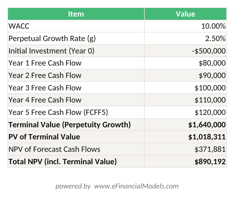
Here is a full numerical build using the perpetuity growth method. Every input appears explicitly so you can replicate this in a blank worksheet.
Assumptions:
- Initial investment (Year 0): −$500,000
- WACC: 10%
- Perpetual growth rate: 2.5%
- Free cash flows: Year 1: $80,000 | Year 2: $90,000 | Year 3: $100,000 | Year 4: $110,000 | Year 5: $120,000
Step 1: Calculate terminal value
TV = $120,000 × (1 + 0.025) ÷ (0.10 − 0.025)TV = $123,000 ÷ 0.075TV = $1,640,000
Step 2: Discount terminal value to present
PV of TV = $1,640,000 ÷ (1.10)⁵ = $1,640,000 ÷ 1.61051 = $1,018,300
Step 3: Apply Excel’s NPV function to forecast cash flows
Enter cash flows in B12:B16 (Years 1–5). In cell B18, enter the terminal value ($1,640,000) added to Year 5’s cash flow, or keep it separate in B17 and include both ranges. The NPV formula:
=NPV(0.10, B12:B16) + NPV(0.10, 0, 0, 0, 0, B17)
Or more cleanly, add the discounted TV directly:
=NPV(0.10, B12:B16) + B17/(1.10)^5
Step 4: Subtract the initial investment
Total NPV = NPV(forecast CFs) + PV(TV) + Initial InvestmentTotal NPV = $341,372 + $1,018,300 − $500,000 = $859,672
The positive NPV of $859,672 confirms this investment creates value at a 10% discount rate. Notice that the PV of terminal value ($1,018,300) accounts for roughly 54% of the combined present value before subtracting the initial investment — illustrating why terminal value assumptions dominate the result.
Total NPV = NPV(forecast CFs) + PV(Terminal Value) + Initial Investment = $341,372 + $1,018,300 − $500,000 = $859,672
Using Excel’s NPV and XNPV Functions: Syntax and Key Differences
Excel provides two functions for present value calculations: NPV for evenly spaced annual periods and XNPV for cash flows on specific calendar dates. Choosing the wrong one introduces systematic discounting errors.
NPV Function Syntax
=NPV(rate, value1, value2, ...)
Critical detail: Excel’s NPV function assumes the first value occurs at the end of period 1, not at period 0. This means you must add the initial investment (as a negative number) outside the function:
=NPV(WACC, B12:B16) + B17/(1+WACC)^5 + B11
Where B11 contains the initial investment as a negative value (e.g., −500000).
XNPV Function Syntax
=XNPV(rate, values, dates)
XNPV discounts each cash flow by the exact number of days between its date and the first date in the series, using the formula: PV = Σ(values ÷ (1 + rate)^((date − first_date) ÷ 365)) (ElyxAI, 2024). The XNPV function requires a minimum of 2 values in the values array, and the first date in the dates array must be the earliest date — any earlier date in the series will cause the function to return a #NUM! error. This makes it far more accurate for real-world deals where cash flows arrive on specific dates rather than neat year-end intervals.
A practical XNPV example uses a 12% discount rate and cash flows of −500,000 followed by five inflows (four payments of 15,000 and one terminal payment of 550,000) across specific dates, illustrating how to include a large terminal cash flow in the function =XNPV(0.12,{−500000,15000,15000,15000,15000,550000}, dates_range) (ElyxAI, 2024).
| Feature | =NPV() | =XNPV() |
|---|---|---|
| Period assumption | Equal annual intervals | Exact calendar dates |
| Date input required | No | Yes (date array) |
| t=0 handling | Must add manually outside function | Include as first value with first date |
| Best use case | Clean annual forecast models | Real transactions with specific payment dates |
| Accuracy for irregular flows | Lower | Higher |
Incorporating Terminal Value into Your NPV Calculation
The terminal value must be discounted back to the present, not simply added to the last forecast year’s cash flow. This is the most common conceptual error in DCF models built by analysts new to the technique.
The correct approach: calculate terminal value using either method above, then divide it by (1 + WACC)ⁿ where n is the final forecast year. In Excel:
=B7*(1+GrowthRate)/(WACC-GrowthRate)/(1+WACC)^5
Or split into two cells for clarity:
- Cell B17:
=B7*(1+GrowthRate)/(WACC-GrowthRate)(terminal value) - Cell B18:
=B17/(1+WACC)^5(present value of terminal value)
Then your total NPV formula becomes:
=NPV(WACC, B12:B16) + B18 + B11
Where B11 is the initial investment (negative). This structure keeps each component visible and auditable.
Common Excel Errors and How to Fix Them
Five specific mistakes account for the majority of DCF errors in practice. Each has a clear fix.
1. Off-by-one period error in NPV function
The =NPV() function discounts value1 as if it occurs at t=1. If you include the Year 0 investment inside the NPV range, it gets discounted one period too many. Fix: always place the initial investment outside the NPV function and add it directly: =NPV(rate, B12:B16) + B11.
2. Forgetting to discount terminal value to present
Calculating terminal value and adding it undiscounted to the NPV sum overstates value by a factor of (1 + WACC)ⁿ. Fix: always divide terminal value by (1 + WACC)^n before adding it to the NPV sum.
3. WACC minus growth rate equals zero or goes negative
If g ≥ WACC, the perpetuity growth formula produces a division-by-zero error or a negative terminal value. Fix: add a validation cell: =IF(WACC-GrowthRate<=0, "ERROR: g ≥ WACC", TV_formula). Keep g at least 2 percentage points below WACC.
4. Circular reference from incorrect cell referencing
Referencing the output NPV cell inside the terminal value formula creates a circular dependency. Fix: structure the model so data flows in one direction only: inputs → cash flows → terminal value → NPV output. Never let an output cell feed back into an input.
5. Inconsistent period conventions
Mixing mid-year and end-of-year discounting within the same model produces errors of 3–7% in present value. Fix: pick one convention (end-of-year is standard for most corporate DCF models) and apply it uniformly across every cash flow and the terminal value discount factor.
Building Sensitivity Analysis for Terminal Value Assumptions
Sensitivity analysis (a technique that shows how the output changes when one or more inputs vary) is essential for any DCF model because terminal value assumptions carry significant uncertainty. Excel’s Data Table feature automates this across a matrix of scenarios.
Two-variable sensitivity table setup:
- Place your base NPV formula in a cell, for example C22.
- In a new block, list WACC values across a row (e.g., 8%, 9%, 10%, 11%, 12% in cells E24:I24).
- List growth rate values down a column (e.g., 1.5%, 2.0%, 2.5%, 3.0%, 3.5% in cells D25:D29).
- In cell D24, enter a reference to your NPV formula:
=C22. - Select the entire block D24:I29, go to Data → What-If Analysis → Data Table.
- Set Row Input Cell to your WACC cell (B2) and Column Input Cell to your growth rate cell (B3).
- Click OK. Excel populates every cell with the NPV under that WACC/growth combination.
For the worked example above (base case: WACC 10%, g 2.5%, NPV $859,672), a sensitivity table typically shows NPV ranging from roughly $600,000 at WACC 12%/g 1.5% to over $1,300,000 at WACC 8%/g 3.5%. That range quantifies the model’s sensitivity and helps you communicate risk to stakeholders. An Excel Data Table can include as many variable values as you want for each of its two inputs, giving you substantial room to expand your scenario grid well beyond the standard 5×5 WACC-versus-growth-rate matrix.
For more advanced multi-scenario modeling, the IRR and NPV modeling templates on EFM include pre-built sensitivity tables you can adapt directly.

A 5×5 sensitivity matrix covering WACC 8–12% and growth rate 1.5–3.5% quantifies the full range of plausible NPV outcomes in under 2 seconds using Excel’s Data Table feature.
Frequently Asked Questions
Why does Excel’s NPV function exclude the initial investment?
Excel’s =NPV(rate, value1, value2, ...) function treats value1 as a cash flow occurring at the end of period 1, not period 0. The initial investment happens at time zero, so it has no discounting applied to it. If you include it inside the NPV range, Excel discounts it by one full period, understating your cost and overstating NPV. The correct structure is always =NPV(rate, CF1:CF5) + Initial_Investment, where the initial investment cell contains a negative number such as −500000. This is one of the most frequently misunderstood behaviors of the function, and it affects every DCF model built in Excel regardless of complexity.
What perpetual growth rate should I use for terminal value?
Most practitioners anchor the perpetual growth rate to long-run nominal GDP growth for the relevant economy. For mature developed markets, that typically falls between 2% and 3%. Using a rate above 4–5% implies the company will eventually grow larger than the entire economy, which is mathematically unsustainable. For a U.S.-based mature industrial company, 2.5% is a common default. For a high-growth technology company, you might use 3%, but you should also run the exit multiple method as a cross-check. The Federal Reserve’s long-run inflation target of 2% provides a useful floor: a growth rate below inflation implies real cash flow decline in perpetuity.
When should I use XNPV instead of NPV in Excel?
Use =XNPV(rate, values, dates) whenever your cash flows do not fall on neat annual intervals. Real-world transactions, project finance deals, and acquisition models often have cash flows on specific calendar dates. XNPV discounts each flow by the exact number of days elapsed since the first date divided by 365, producing a more accurate present value than NPV’s assumption of equal annual spacing. For example, a cash flow received 18 months after the start date gets discounted by (1 + rate)^(548/365) = (1 + rate)^1.5, not by (1 + rate)^1 or (1 + rate)^2. The syntax is =XNPV(0.12, B11:B16, C11:C16) where column B holds cash flow values and column C holds the corresponding dates.
How do I validate that my terminal value is reasonable?
Run both the perpetuity growth method and the exit multiple method and compare results. If they diverge by more than 20–30%, revisit your assumptions. For the perpetuity growth result, back-solve for the implied exit multiple: Implied Multiple = Terminal Value ÷ EBITDA₅. If the implied multiple is 25× for a mature industrial company where peers trade at 7–9×, your growth rate is too high. For the exit multiple result, back-solve for the implied perpetual growth rate: g = WACC − (FCFF₆ ÷ Terminal Value). If the implied g exceeds 5%, your multiple is too aggressive. This cross-check takes under 5 minutes and catches the majority of terminal value errors before they reach a client or investment committee.
What WACC range is typical for DCF models?
WACC varies significantly by industry, company size, and capital structure. For large-cap U.S. public companies, WACC typically falls between 7% and 12%. Technology companies with higher equity risk premiums often use 10–14%. Regulated utilities with stable cash flows may use 5–8%. Emerging market companies add a country risk premium of 2–5 percentage points on top of the base WACC. For private companies without observable market betas, practitioners often apply a size premium of 1–4% above the comparable public company WACC. Always document your WACC derivation in the assumptions section of your model so reviewers can challenge individual components rather than the blended rate.
Can terminal value ever be negative?
Yes, and it always signals a model error. Terminal value using the perpetuity growth method equals FCFF₅ × (1 + g) ÷ (WACC − g). If WACC is less than g, the denominator is negative, producing a negative terminal value. This is mathematically impossible for a going-concern business: no rational buyer pays a negative price for future cash flows. The fix is to ensure g is always strictly less than WACC. Add a validation check in your model: =IF(WACC-GrowthRate<=0,"INVALID: g must be < WACC",TV_formula). A negative terminal value from the exit multiple method is also impossible since EBITDA and multiples are both positive by definition.
How do I build a two-variable sensitivity table for NPV in Excel?
Excel’s Data Table feature (found under Data → What-If Analysis → Data Table) creates a matrix of NPV outcomes across combinations of two inputs, typically WACC and perpetual growth rate. Set up a grid with WACC values across the top row and growth rate values down the left column. Place a reference to your NPV formula in the top-left corner of the grid. Select the entire grid, open Data Table, assign the row input cell to your WACC cell and the column input cell to your growth rate cell, then click OK. Excel recalculates NPV for every combination instantly. For the worked example in this article, a 5×5 grid covering WACC from 8–12% and g from 1.5–3.5% produces 25 NPV scenarios in under 2 seconds, giving you a complete picture of value sensitivity without writing a single additional formula.
Conclusion
Calculating NPV with terminal value in Excel requires three things done correctly: an accurate terminal value formula (perpetuity growth or exit multiple), proper discounting of that terminal value back to the present, and correct use of Excel’s NPV function with the initial investment added outside the range. Terminal value dominates DCF results, often representing 60–80% of total enterprise value, so every assumption deserves explicit validation and sensitivity testing.
For NPV modeling and terminal value work, a pre-built template saves hours of setup and eliminates structural errors. The Excel financial models library at EFM includes DCF templates with built-in sensitivity tables and error-checking formulas. For multi-project analysis, the IRR modeling template extends these techniques across parallel investment scenarios.
I recommend downloading the EFM DCF Valuation Model with 3 Years Actual and 5 Years Forecast as your starting template. It includes a pre-structured assumptions block, named ranges for WACC and growth rate, a two-variable sensitivity table, and validation checks for the WACC-minus-growth-rate condition, so you can focus on the analysis rather than the architecture.