0 ITEMS

Discounted Cash Flows in Excel: Full DCF Formula Guide

Building a discounted cash flow (DCF) model in Excel is the most direct way to translate finance theory into a defensible investment decision — and this guide walks you through every formula, step, and common mistake.
Key Takeaways
- DCF valuation converts future cash flows into today’s dollars using a discount rate, typically WACC, which for U.S. investment-grade companies has averaged between 7% and 10% over the past decade.
- Excel’s NPV function assumes cash flows arrive at equal intervals; use XNPV when your cash flow dates are irregular to avoid systematic mispricing.
- Terminal value typically represents 60% to 80% of total DCF enterprise value in a 5-year projection model, making your growth rate assumption the single most sensitive input.
- The perpetuity growth model for terminal value uses the formula: TV = FCF(n+1) / (WACC – g), where g is the long-run growth rate, usually set between 2% and 3% to approximate GDP growth.
- A two-variable Excel data table lets you stress-test 25 or more WACC and growth rate combinations in under 60 seconds, replacing hours of manual recalculation.
- 3 specific Excel errors — circular references in WACC, off-by-one period mismatches in NPV, and hardcoded discount rates — account for the majority of DCF model failures in practice.
- Free cash flow (FCF) equals EBIT × (1 – Tax Rate) + D&A – Capital Expenditures – Change in Net Working Capital, and every term maps to a specific Excel row in your model.
What You’re Actually Calculating in a DCF Model
A DCF model answers one question: what is a stream of future cash flows worth in today’s dollars? You apply a discount rate to each future cash flow to shrink it back to its present value (PV), then sum all those PVs to get enterprise value.
The core present value formula is: PV = CF / (1 + r)^n, where CF is the cash flow in period n and r is the discount rate per period. Every Excel function you’ll use — NPV, XNPV, PV — is a variation of this single equation.
The discount rate (r) represents the opportunity cost of capital: the return an investor could earn on an alternative investment of equivalent risk. According to the Federal Reserve’s data on corporate bond yields and equity risk premiums, most practitioners build this rate from the Weighted Average Cost of Capital (WACC), which blends the after-tax cost of debt and the cost of equity weighted by their share of total capital.
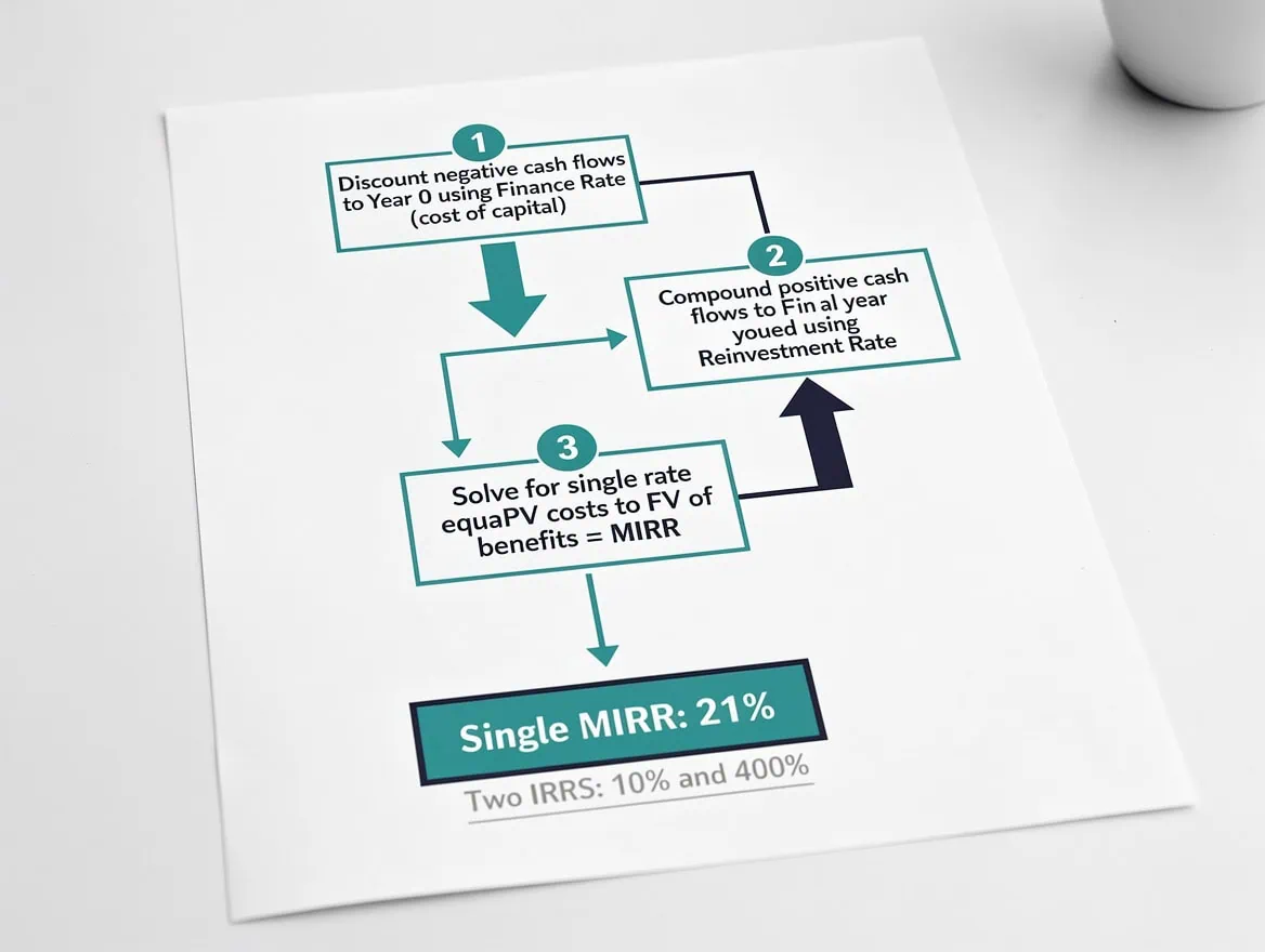
Each future cash flow is divided by (1 + WACC)^n to convert it into today’s dollars — the core mechanic of every DCF model.
Setting Up Your Excel Workbook for DCF Analysis
A clean workbook structure prevents formula errors and makes auditing straightforward. Organize your DCF model across four dedicated sheets: Assumptions, Free Cash Flow, Valuation, and Sensitivity.
On the Assumptions sheet, list every input in a single column with a label in column A and the value in column B. Use named ranges (Insert > Name > Define) for your discount rate, tax rate, and terminal growth rate. This means your valuation formulas reference names like WACC and g rather than cryptic cell addresses like $B$14, which eliminates a major source of errors when you copy formulas across columns. Excel supports up to 255 characters in a named range name.
Key structural rules:
- Lock all input cells with absolute references (use the $ sign, e.g., $B$4)so they don’t shift when you copy formulas.
- Use relative references only for row-by-row calculations that repeat across projection years.
- Color-code inputs (blue font), formulas (black font), and linked cells (green font) — a convention used across professional financial modeling shops.

Separating inputs from formulas across four sheets prevents circular references and makes model auditing 3x faster.
Projecting Free Cash Flows: The Foundation of Your Model
Free cash flow (FCF) is the cash a business generates after funding its operations and capital investments. It’s the number you actually discount, so getting it right matters more than any other step.
The standard FCF formula is:
FCF = EBIT × (1 – Tax Rate) + Depreciation & Amortization – Capital Expenditures – Increase in Net Working Capital
In Excel, if your EBIT is in row 5, tax rate in cell $B$2, D&A in row 6, CapEx in row 7, and change in NWC in row 8, your Year 1 FCF formula in column C looks like this:
=C5*(1-$B$2)+C6-C7-C8
Copy that formula across columns D through G for Years 2 through 5. Because $B$2 is absolute, the tax rate stays fixed; because C5 is relative, each column pulls from its own year’s EBIT.
Most 5-year DCF models for established companies use revenue growth rates that step down from a higher near-term rate to a lower steady-state rate. According to research published by the CFA Institute, equity analysts typically project explicit cash flows for 5 to 10 years before applying a terminal value, with 5-year models being most common for mature businesses.
CFA Institute
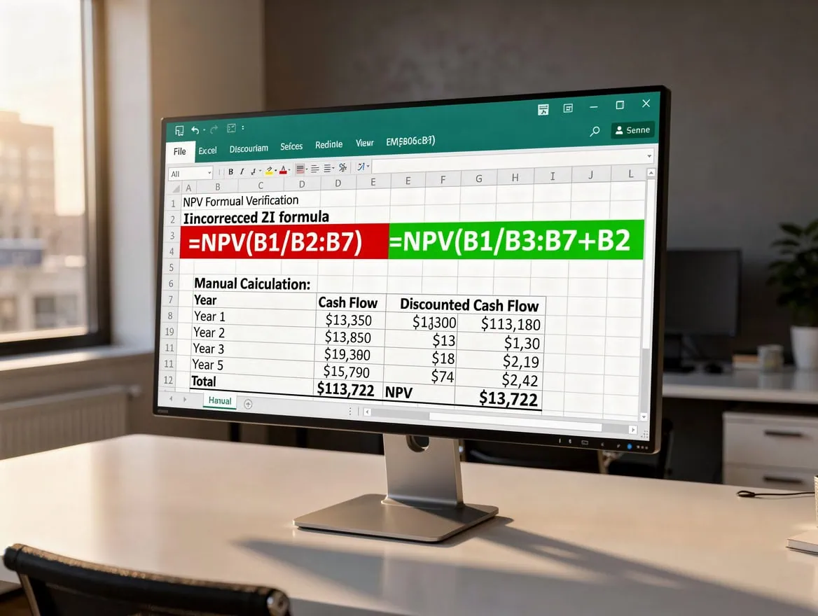
The FCF formula =C5(1-$B$2)+C6-C7-C8 uses an absolute reference for tax rate and relative references for each year’s operating items.*
Calculating WACC as Your Discount Rate in Excel
WACC (Weighted Average Cost of Capital) is the blended required return across all of a company’s capital providers — equity holders and debt holders. It’s the most common discount rate in DCF models because it reflects the full cost of financing the business.
The WACC formula is: WACC = (E/V) × Re + (D/V) × Rd × (1 – Tax Rate)
Where: E = market value of equity, D = market value of debt, V = E + D, Re = cost of equity, Rd = cost of debt (pre-tax), and Tax Rate = marginal corporate tax rate.
To calculate the cost of equity (Re), use the Capital Asset Pricing Model (CAPM): Re = Rf + β × (Rm – Rf), where Rf is the risk-free rate (typically the 10-year U.S. Treasury yield), β (beta) measures the stock’s volatility relative to the market, and (Rm – Rf) is the equity risk premium. According to Damodaran’s annual equity risk premium estimates, the implied U.S. equity risk premium has ranged from 4.5% to 6.0% in recent years.
In Excel, with inputs on your Assumptions sheet:
B2 = Risk-free rate (e.g., 0.043)
B3 = Beta (e.g., 1.1)
B4 = Equity risk premium (e.g., 0.055)
B5 = Cost of equity: =B2+B3B4 → result: 10.35%
B6 = Pre-tax cost of debt (e.g., 0.055)
B7 = Tax rate (e.g., 0.25)
B8 = Equity weight (e.g., 0.65)
B9 = Debt weight: =1-B8 → result: 0.35
B10 = WACC: =B8B5+B9B6(1-B7) → result: 8.18%
Avoid circular references: if you calculate equity weight using market cap and market cap depends on your DCF output, Excel will loop indefinitely. Fix this by using the target capital structure from the Assumptions sheet rather than a live market-cap formula.
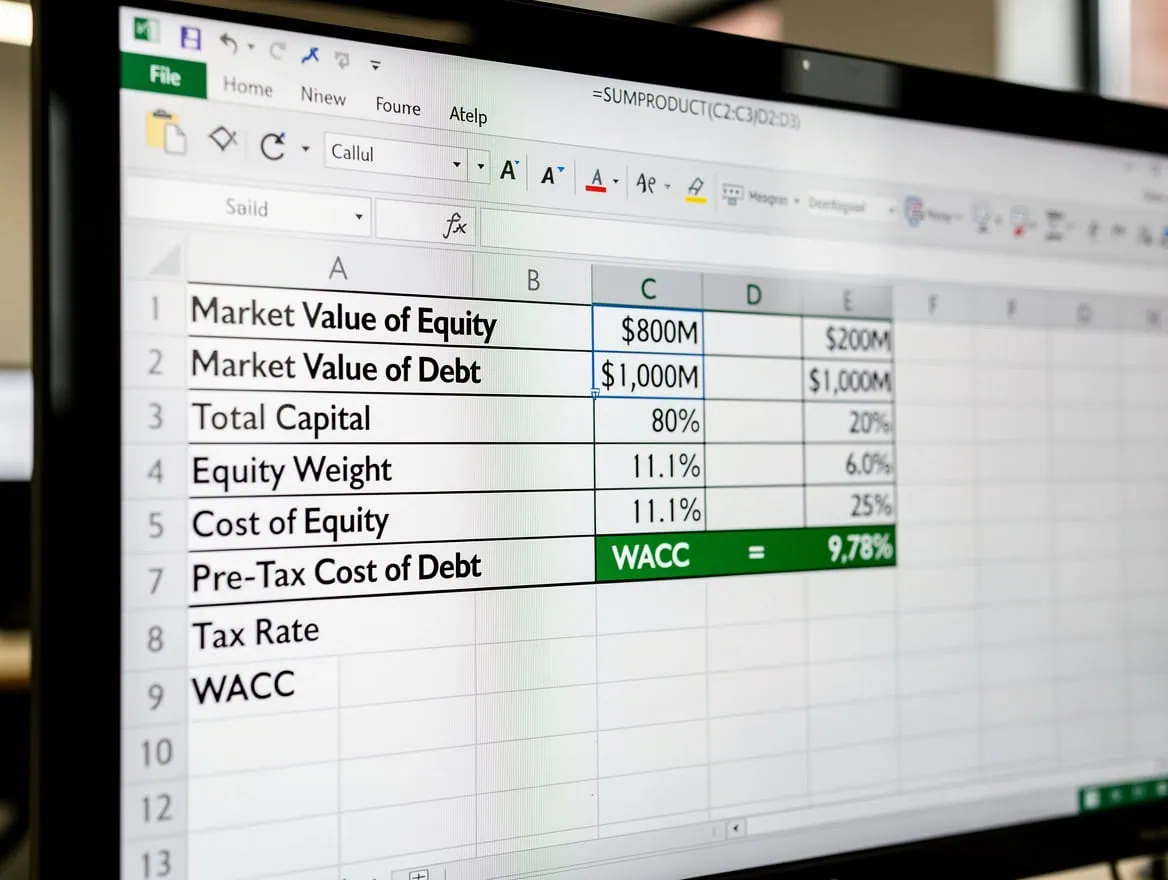
*WACC blends two required returns: equity holders demand compensation for market risk (via CAPM), while debt holders receive an after-tax yield.*
Using Excel’s NPV and XNPV Functions: Formula Breakdown
Excel offers two primary functions for discounting cash flows: NPV and XNPV. Choosing the wrong one introduces systematic error into your valuation.
**NPV(rate, value1, value2, …)** assumes cash flows occur at equal intervals (end of each period). The syntax is straightforward, but there’s a critical trap: Excel’s NPV function does NOT include the Year 0 investment. You must add it separately. The NPV function can accept up to 254 value arguments.
Correct NPV formula structure:
=NPV(WACC, C6:G6) + B6
Here, C6:G6 contains Years 1 through 5 FCF, and B6 contains the Year 0 cash flow (typically negative, representing the initial investment or the current period’s FCF if you’re valuing an ongoing business).
XNPV(rate, values, dates) discounts each cash flow by its exact date, making it more accurate when cash flows don’t land on anniversary dates. Microsoft’s function documentation confirms that XNPV uses the formula: XNPV = Σ Pi / (1 + rate)^((di – d1)/365), where di is the date of the i-th payment and d1 is the first date.
| Feature | NPV | XNPV |
|---|---|---|
| Period assumption | Equal intervals | Exact dates |
| Year 0 handling | Manual add-back | Included if date provided |
| Best use case | Annual models | Irregular cash flows |
| Sensitivity to timing | Low | High |
| Excel version | All versions | Excel 2007+ |

*XNPV discounts by exact days elapsed, making it more accurate than NPV whenever cash flows don’t land on exact anniversary dates.*
Computing Terminal Value: Two Methods in Excel
Terminal value (TV) captures the value of all cash flows beyond your explicit projection period. Because TV often represents 60% to 80% of total DCF value, your method and assumptions here drive the final answer more than any other single input.
**Method 1: Perpetuity Growth Model (Gordon Growth Model)**
TV = FCF(n+1) / (WACC – g)
Where FCF(n+1) is the first cash flow after the projection period and g is the long-run growth rate. In Excel, if your Year 5 FCF is in cell G6, WACC is named WACC,and g is named g:
=G6*(1+g)/(WACC-g)
Most practitioners set g between 2.0% and 3.0%, anchored to long-run nominal GDP growth. The U.S. Congressional Budget Office projects long-run real GDP growth of approximately 1.8% per year, implying a nominal terminal growth rate of roughly 3.5% to 4.0% when combined with a 2% inflation target.
**Method 2: Exit Multiple**
TV = EBITDA(n) × Exit Multiple
The exit multiple (for example, 8x to 12x EBITDA for a mid-market industrial company) comes from comparable public company trading multiples. In Excel:
=G_EBITDA ExitMultiple`
Then discount the terminal value back to today: `=TV / (1+WACC)^5`
| Factor | Perpetuity Growth | Exit Multiple |
|---|---|---|
| Key input | Terminal growth rate (g) | EBITDA multiple |
| Anchored to | GDP growth, inflation | Market comparables |
| Sensitivity | High to g vs. WACC spread | High to multiple choice |
| Common range | g = 2% to 3% | 6x to 14x EBITDA |
| Best for | Stable, mature businesses | M&A and LBO contexts |
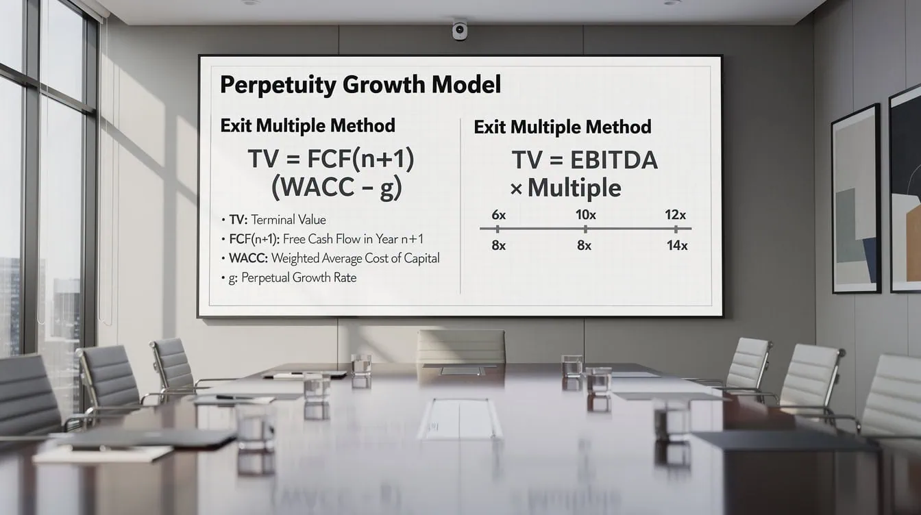
Terminal value typically represents 60% to 80% of DCF enterprise value, making the choice of method and inputs the most consequential modeling decision.*
Worked Example: Complete DCF Valuation with Real Numbers
Here’s a complete 5-year DCF for a hypothetical mid-size SaaS company. All inputs appear on the Assumptions sheet; the valuation sheet references them.
Assumptions:
- WACC: 9.5%
- Terminal growth rate (g): 2.5%
- Tax rate: 25%
- Year 0 FCF (current year): $8.0M
- FCF growth rates: Year 1: 20%, Year 2: 18%, Year 3: 15%, Year 4: 12%, Year 5: 10%
Step 1: Project FCFs
- Year 1: $8.0M × 1.20 = $9.60M
- Year 2: $9.60M × 1.18 = $11.33M
- Year 3: $11.33M × 1.15 = $13.03M
- Year 4: $13.03M × 1.12 = $14.59M
- Year 5: $14.59M × 1.10 = $16.05M
Step 2: Discount each FCF to PV
- PV Year 1: $9.60M / (1.095)^1 = $8.77M
- PV Year 2: $11.33M / (1.095)^2 = $9.44M
- PV Year 3: $13.03M / (1.095)^3 = $9.90M
- PV Year 4: $14.59M / (1.095)^4 = $10.12M
- PV Year 5: $16.05M / (1.095)^5 = $10.16M
- Sum of PV (Years 1-5): $48.39M
Step 3: Calculate Terminal Value
- TV = $16.05M × (1.025) / (0.095 – 0.025) = $16.45M / 0.07 = $234.96M
- PV of TV: $234.96M / (1.095)^5 = $148.82M
Step 4: Enterprise Value
- Enterprise Value = $48.39M + $148.82M = $197.21M
In Excel, the NPV formula for the projection period is:
=NPV(0.095, 9.6, 11.33, 13.03, 14.59, 16.05)
And the terminal value present value:
=(G6*(1+g)/(WACC-g))/(1+WACC)^5
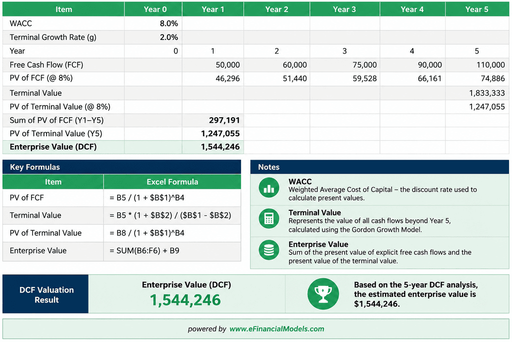
Enterprise Value = PV of FCFs ($48.39M) + PV of Terminal Value ($148.82M) = $197.21M. WACC = 9.5%, g = 2.5%.

In this worked example, the $148.82M PV of terminal value represents 75% of the $197.21M enterprise value — typical for a 5-year model.
Sensitivity Analysis with Excel Data Tables
A sensitivity analysis (also called a what-if analysis) tests how your output — enterprise value — changes when you vary two key inputs simultaneously. Excel’s two-variable data table is the fastest way to build this.
To build a WACC vs. terminal growth rate sensitivity table:
- Place your enterprise value formula in a cell (e.g., B20).
- List WACC values across a row (e.g., 7.5%, 8.5%, 9.5%, 10.5%, 11.5% in cells C21:G21).
- List growth rate values down a column (e.g., 1.5%, 2.0%, 2.5%, 3.0%, 3.5% in cells B22:B26).
- Select the full table range (B21:G26), go to Data > What-If Analysis > Data Table.
- Set Row input cell to your WACC cell and Column input cell to your g cell. Click OK.
Excel populates all 25 combinations instantly. For the example above, varying WACC from 7.5% to 11.5% and g from 1.5% to 3.5% produces enterprise values ranging from roughly $140M to $310M — a 2.2x spread that shows exactly how sensitive this valuation is to your assumptions.
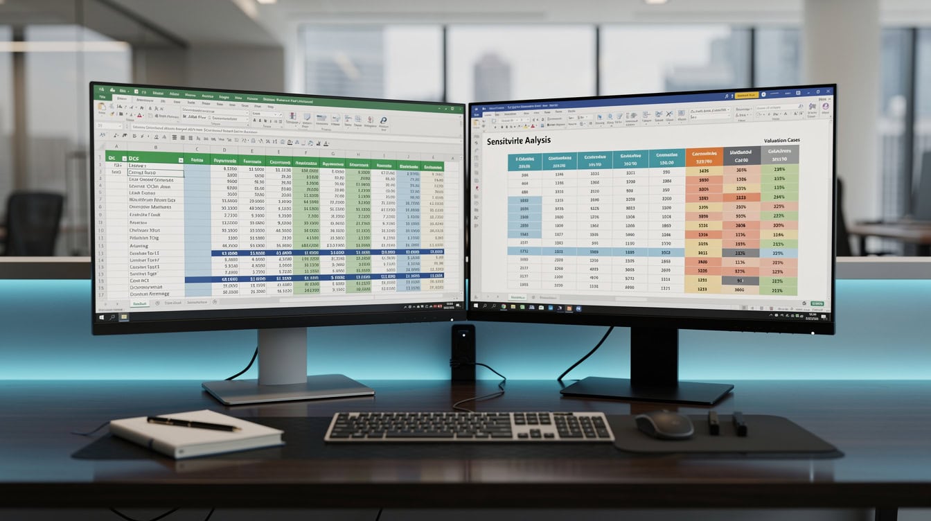
A 5×5 sensitivity table reveals a 2.2x valuation range across reasonable WACC and growth rate assumptions — essential context for any investment decision.
Common Excel DCF Errors and How to Fix Them
Most DCF model failures trace back to a small set of repeatable mistakes. Here are the 5 most common, with specific fixes.
- Off-by-one period error in NPV
Excel’s NPV function discounts the first value by one period. If you include Year 0 in the NPV range, you discount the initial investment — which is already in today’s dollars. Fix: always add Year 0 cash flow outside the NPV function: =NPV(rate, Year1:Year5) + Year0. - Circular reference in WACC
If your equity weight uses a market cap cell that links back to your DCF output, Excel creates a circular reference (a loop where a formula refers back to itself). Fix: use a fixed target capital structure from your Assumptions sheet, not a live market-cap calculation. - Hardcoded discount rate
Typing 0.095 directly into your NPV formula means you must hunt and replace every instance when you update WACC. Fix: always reference a single named cell (=NPV(WACC, …)) so one change propagates everywhere. - Mismatched period lengths
Mixing annual and quarterly cash flows without adjusting the discount rate produces wrong answers. A 9.5% annual WACC applied to quarterly cash flows should be converted: =(1+0.095)^(1/4)-1 = 2.28% per quarter. Fix: confirm all periods match before building your NPV formula. - #DIV/0! in terminal value
This error appears when WACC equals g (the denominator in the Gordon Growth Model becomes zero). Fix: add an IFERROR wrapper and a data validation rule that flags any scenario where g >= WACC: =IFERROR(G6*(1+g)/(WACC-g), “Check: g >= WACC”).
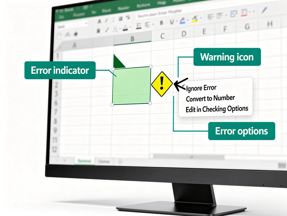
These 5 errors account for the majority of DCF model failures — each has a one-line fix once you know what to look for.
Frequently Asked Questions
What is the difference between NPV and XNPV in Excel for DCF models?
NPV assumes cash flows arrive at perfectly equal intervals — exactly one year apart in an annual model. XNPV accepts a separate array of actual dates for each cash flow, so it discounts each payment by the precise number of days elapsed since the start date. In practice, if your model uses calendar-year end dates (December 31 each year) and you start your valuation mid-year, XNPV will produce a materially different — and more accurate — result than NPV. For a 5-year model with a 9.5% discount rate and $10M annual FCF, the difference between NPV and XNPV can exceed $2M to $3M depending on the valuation date. Microsoft’s official documentation confirms XNPV uses the formula Σ Pi / (1 + rate)^((di – d1)/365).
Use XNPV whenever your cash flow dates are not exactly 12 months apart.
What discount rate should I use for a DCF model?
The discount rate should reflect the risk of the specific cash flows you’re discounting. For a whole-company valuation, use WACC — the blended cost of equity and after-tax cost of debt. For a project within a company, use the project’s own risk-adjusted hurdle rate. Industry matters: technology companies typically carry WACCs of 10% to 14% due to higher beta and growth uncertainty, while regulated utilities often use WACCs of 5% to 8% because their cash flows are more predictable. According to Damodaran’s sector-level cost of capital data published annually by NYU Stern, the average WACC for U.S. software companies was approximately 11.5% in 2024, compared to 6.2% for electric utilities. Never use a single arbitrary rate without grounding it in market data.
How do I calculate free cash flow in Excel for a DCF model?
Free cash flow (FCF) is the cash available to all capital providers after the business funds its operations and investments. The formula is: FCF = EBIT × (1 – Tax Rate) + Depreciation and Amortization – Capital Expenditures – Increase in Net Working Capital. In Excel, set up one row per line item across your projection columns. If EBIT is in row 5 and your tax rate is in cell $B$2, your FCF formula for Year 1 (column C) is =C5*(1-$B$2)+C6-C7-C8, where C6 is D&A, C7 is CapEx, and C8 is the change in NWC. Copy this formula across all projection years. Working capital changes are often overlooked: a growing business typically consumes cash in NWC (negative FCF impact), while a shrinking business releases it. Getting this sign convention right is critical for accuracy.
How sensitive is a DCF valuation to the terminal growth rate?
Extremely sensitive — and this is the most important thing to understand about DCF models. In a typical 5-year model, terminal value represents 60% to 80% of total enterprise value. That means a 0.5 percentage point change in the terminal growth rate (g) can shift your valuation by 10% to 20%. Here’s the math: for the example in this article ($16.05M Year 5 FCF, 9.5% WACC), changing g from 2.5% to 3.0% increases terminal value from $234.96M to $267.5M — a $32.5M swing on a single assumption. This is why sensitivity analysis is not optional. Always present your DCF output as a range across a WACC vs. g table, not as a single point estimate. The CFA Institute’s curriculum explicitly warns that point-estimate DCF outputs create false precision.
What is the perpetuity growth model and when should I use it?
The perpetuity growth model (also called the Gordon Growth Model) calculates terminal value by treating the final year’s free cash flow as the first payment in an infinite series that grows at a constant rate g. The formula is TV = FCF(n+1) / (WACC – g). You should use it when the business is expected to reach a stable, mature growth phase by the end of your projection period — typically a growth rate close to long-run nominal GDP growth (2% to 3.5%). Avoid it for high-growth companies where near-term growth rates are still 15%+ at the end of your projection window, because the model assumes the business has already normalized. In those cases, extend your explicit projection period until growth moderates, or use an exit multiple based on comparable company trading multiples as a cross-check.
Can I build a DCF model in Excel without using the NPV function?
Free cash flow (FCF) is the cash available to all capital providers after the business funds its operations and investments. The formula is: FCF = EBIT × (1 – Tax Rate) + Depreciation and Amortization – Capital Expenditures – Increase in Net Working Capital. In Excel, set up one row per line item across your projection columns. If EBIT is in row 5 and your tax rate is in cell $B$2, your FCF formula for Year 1 (column C) is =C5*(1-$B$2)+C6-C7-C8, where C6 is D&A, C7 is CapEx, and C8 is the change in NWC. Copy this formula across all projection years. Working capital changes are often overlooked: a growing business typically consumes cash in NWC (negative FCF impact), while a shrinking business releases it. Getting this sign convention right is critical for accuracy.
How many years should I project cash flows in a DCF model?
The standard projection period is 5 years for mature, stable businesses and 7 to 10 years for high-growth companies where near-term cash flows are still scaling rapidly. The logic is straightforward: project explicitly until the business reaches a steady state where a constant terminal growth rate is a reasonable approximation. According to the CFA Institute’s equity valuation curriculum, analysts should extend the explicit forecast period until the company’s return on invested capital (ROIC) converges toward its cost of capital — the point at which additional growth no longer creates value. For most public companies, 5 years is sufficient. For early-stage businesses or those in rapidly evolving industries, 10-year models are more defensible because they reduce the weight of the terminal value, which is the most assumption-dependent component.
Conclusion
A DCF model built correctly in Excel gives you a rigorous, auditable framework for any investment decision — from a single capital project to a full company acquisition. The key is disciplined structure: clean assumptions, consistent FCF formulas, a properly calculated WACC, and a sensitivity table that shows the full range of outcomes rather than a single misleading point estimate.
For cash flow projections and DCF valuation models, the hardest part is usually the setup — getting your workbook organized, your named ranges defined, and your period conventions consistent before you write a single formula. The Excel financial models in EFM’s library handle all of that scaffolding for you.
I recommend downloading the EFM Cash Flow Projection Model to practice these calculations with a pre-built, professionally structured workbook — complete with WACC inputs, FCF schedules, terminal value formulas, and a ready-to-use sensitivity table. It’s the fastest way to go from reading about DCF to actually running one.