0 ITEMS

Cash-Flow Forecasting for Banks: Strategic Model Guide
Bank cash-flow forecasting was built on an assumption that no longer holds: that the bank is the primary lender to its own market. Private credit now funds the majority of mid-sized corporate borrowers, Basel III makes those loans expensive to hold, and fee-based origination is replacing spread income as the growth engine. This guide shows how to rebuild a bank’s strategic cash-flow model around that reality, with a six-module framework, worked capital and customer-value examples, and a phased plan for moving from a legacy NIM model to a fee-based one.
Key Takeaways
- Private credit AUM hit nearly $2 trillion in 2024 and is projected to reach $4 trillion by 2028, forcing banks to rethink every line item in their cash-flow forecasts.
- Non-bank lenders now originate more than 60% of corporate loans under $100 million, making the middle-market segment a structural loss leader for traditionally modeled banks.
- Basel III capital charges on sub-$100M corporate loans create a measurable cost disadvantage that must be explicitly modeled, not assumed away.
- Banks using precision, data-driven engagement models lift customer engagement by 20 to 30 percentage points and increase customer value by 10 to 25%, according to McKinsey’s Global Banking Annual Review.
- The strategic pivot from net interest margin (NIM) to origination-as-a-service fee revenue changes the shape of a bank’s cash-flow forecast entirely: lower loan balances, higher fee lines, different capital consumption.
- A modern bank cash-flow model must include at least five components: capital allocation under Basel III, fee revenue projections, customer lifetime value (CLV), credit migration scenarios, and competitive displacement assumptions.
- Transitioning a legacy NIM-focused model to a fee-based framework takes three structured phases and typically requires rebuilding the revenue driver tree from scratch.
The Competitive Imperative: Why Bank Modeling Must Evolve Now
Traditional bank cash-flow forecasting assumes the bank is the primary lender. That assumption is now structurally broken in the middle market, and any model that ignores it will systematically overstate loan volume and understate margin compression.
Private credit assets under management reached nearly $2 trillion in 2024, growing nearly tenfold from pre-global financial crisis levels, and are projected to surpass $4 trillion by 2028 (Wolters Kluwer). That growth did not happen in a vacuum: it came directly at the expense of bank lending economics. Non-bank lenders now originate more than 60% of corporate loans under $100 million in the middle-market segment (Wolters Kluwer). A bank model that projects middle-market loan growth using historical bank origination rates is projecting into a market the bank no longer dominates.
The implication for FP&A teams is direct: your revenue driver tree, your capital consumption schedule, and your customer value assumptions all need to be rebuilt around the competitive reality, not the historical baseline.

Understanding the Market Context: Private Credit’s $2 Trillion Challenge
The private credit expansion is not a cyclical shift. It is a structural reallocation of credit intermediation away from regulated balance sheets toward unregulated capital pools, and it has specific implications for how you model each loan segment.
Private credit funds operate without the capital adequacy requirements that govern banks. They can price sub-$100M corporate loans more aggressively because they do not carry the same regulatory capital charge per dollar of exposure. For a bank’s cash-flow model, this means the addressable market for traditional balance-sheet lending in the middle market is shrinking in real terms, even when total credit demand grows.
Your model should segment the loan book into at least three competitive tiers:
- Large corporate (above $500M): Banks retain strong competitive position; model using historical origination share with modest compression.
- Mid-market ($100M to $500M): Contested territory; apply a 10-15% annual origination share haircut in base case.
- Sub-$100M middle market: Non-bank dominated; model origination volume as fee-based referral income rather than on-balance-sheet lending.
This segmentation alone changes the shape of a five-year cash-flow forecast materially. Loan balance growth slows, NIM contribution shrinks, and fee income must compensate.

The Basel III Capital Constraint and Its Modeling Implications
Basel III (the international bank capital adequacy framework finalized by the Basel Committee on Banking Supervision) imposes risk-weighted capital charges that make sub-$100M corporate lending structurally expensive for banks relative to non-bank competitors.
Under the standardized approach, unrated corporate exposures carry a 100% risk weight, meaning a bank must hold approximately 8% Tier 1 capital against each dollar lent. For a $50M corporate loan, that is $4M in capital tied up at a cost of equity typically running 10-14% for U.S. banks. The implied capital cost alone is $400,000 to $560,000 annually before any credit loss provision. Non-bank lenders face no equivalent regulatory capital floor, allowing them to offer tighter spreads and still generate acceptable returns for their investors.
Banks are increasingly shifting their commercial lending role toward origination-as-a-service, focusing revenue on fee-based economics rather than net interest margin, precisely because of these Basel III capital charges on sub-$100 million corporate loans (Wolters Kluwer).
In your model, Basel III constraints should appear as explicit inputs, not background assumptions:
- Risk-weighted asset (RWA) density: Express each loan segment as a percentage of notional balance (e.g., 100% for unrated corporate, 75% for investment-grade corporate).
- Capital cost per segment: Multiply RWA density by the cost of equity to get the annual capital charge per dollar of exposure.
- Return on RWA: Use this as the primary profitability metric for lending segments, replacing simple NIM.

Quantifying the Precision Modeling Advantage: 20-30% Engagement Gains
Precision modeling does not just improve forecast accuracy. It directly drives the customer engagement outcomes that feed back into revenue projections.
Leading banks using precision, data-driven models are lifting customer engagement by 20 to 30 percentage points (McKinsey & Company, Global Banking Annual Review). The same research shows these banks are increasing customer value by 10 to 25% (McKinsey & Company, Global Banking Annual Review). These are not soft metrics: they translate directly into fee revenue per relationship, cross-sell conversion rates, and customer lifetime value, all of which are explicit line items in a modern bank cash-flow model.
Here is how to incorporate these figures into your projection assumptions:
- Engagement lift input: Add a “precision model adoption” toggle in your model. In the base case (no precision model), use historical engagement rates. In the upside case, apply a 20-30 percentage point lift to the engagement rate driving fee product penetration.
- Value increase input: Apply a 10-25% multiplier to your CLV (customer lifetime value) calculation for the customer cohort served by precision engagement tools.
- Sensitivity table: Run a two-variable sensitivity showing fee revenue outcomes across engagement lift (0%, 10%, 20%, 30%) and CLV improvement (0%, 10%, 15%, 25%).
This structure lets you present the precision modeling investment as a quantified revenue driver, not a vague technology benefit.

Modeling the Strategic Pivot: From NIM to Fee-Based Origination
The shift from net interest margin to origination-as-a-service is the single biggest structural change in bank revenue modeling, and it requires rebuilding the revenue driver tree rather than simply adding a fee line.
In a NIM-focused model, revenue is a function of loan balances multiplied by spread. In an origination-as-a-service model, revenue is a function of origination volume multiplied by fee rate, with the loan itself sitting on a non-bank balance sheet. The bank earns a structurally different cash flow: lower, more predictable, capital-light, but also more volume-sensitive.
Comparison: NIM Model vs. Fee-Based Origination Model
| Dimension | Traditional NIM Model | Fee-Based Origination Model |
|---|---|---|
| Revenue driver | Loan balance × spread | Origination volume × fee rate |
| Capital consumption | High (RWA-intensive) | Low (off-balance-sheet) |
| Revenue volatility | Rate-sensitive | Volume-sensitive |
| Credit risk exposure | Full on-balance-sheet | Minimal (sold/referred) |
| Margin profile | 2.5-3.5% NIM typical | 0.5-1.5% origination fee |
| Scalability | Capital-constrained | Operationally constrained |
| Forecast complexity | Balance sheet + P&L | P&L only (simpler) |
The fee rate range of 0.5-1.5% on origination volume is the key modeling input. A bank originating $2B in sub-$100M corporate loans annually at a 1% fee earns $20M in fee revenue with near-zero capital consumption, compared to holding those loans on balance sheet at a 2.5% NIM but consuming roughly $160M in Tier 1 capital.

Framework: Building a Modern Bank Strategic Cash-Flow Model
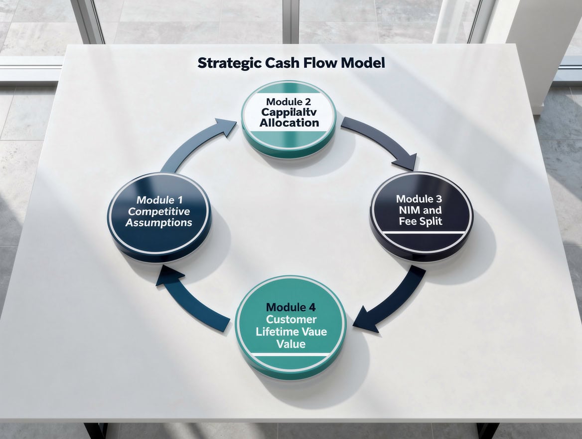
A modern bank strategic model has six core modules. Each module feeds the next, and the output is a fully integrated cash-flow forecast that reflects competitive, regulatory, and strategic realities.
Module 1: Loan Segment Competitive Assumptions
Define origination share by segment (large corporate, mid-market, sub-$100M) with explicit non-bank competition haircuts. This drives loan balance projections.
Module 2: Capital Allocation Schedule
Map each loan segment to its RWA density and calculate capital consumption. This constrains loan growth and determines the return on equity for each segment.
Module 3: NIM and Fee Revenue Split
Project NIM revenue from retained loans and fee revenue from originated-and-sold or referred loans. The mix shifts over the forecast period as the origination-as-a-service model scales.
Module 4: Customer Lifetime Value Model
Calculate CLV per customer cohort using engagement rate, product penetration, average revenue per product, and churn rate. Apply the 10-25% precision model uplift as a scenario variable.
Module 5: Credit Migration and Provision Scenarios
Model credit quality migration as non-bank competition selects the best credits (adverse selection risk for banks). Provision rates on retained loans may rise as the credit pool quality declines.
Module 6: Integrated Cash-Flow Statement
Consolidate operating cash flows (NIM + fees + service charges), investing cash flows (loan originations net of repayments), and financing cash flows (capital raises, dividends) into a three-statement model.
Middle-Market Lending: Modeling Under 60%+ Non-Bank Competition
The sub-$100M middle market requires a fundamentally different modeling approach than large corporate lending, because the competitive dynamics are inverted: non-banks are the incumbents, and banks are the challengers.
For this segment, your model should project three scenarios:
- Retreat scenario: Bank exits on-balance-sheet lending below $100M entirely. Model the capital release and redeploy it into higher-return segments. Fee income from referral arrangements replaces NIM.
- Selective retention scenario: Bank retains only investment-grade or relationship-anchored credits below $100M. Apply a 40-50% volume reduction from historical origination levels and a 15-20 basis point NIM compression from competitive pricing pressure.
- Origination-as-a-service scenario: Bank originates at full historical volume but sells or syndicates 70-80% to non-bank partners, retaining a 0.75-1.25% origination fee. Capital consumption drops by 70-80% for this segment.
The origination-as-a-service scenario typically generates the highest risk-adjusted return on equity for this segment, which is why it is the direction the industry is moving.
Customer Value Modeling: Incorporating 10-25% Improvement Assumptions
Customer lifetime value (CLV) in banking is the present value of all future net revenue from a customer relationship, discounted at the bank’s cost of capital. Precision engagement models improve CLV through two mechanisms: higher product penetration per customer and lower churn rates.
Worked Example: CLV Calculation with Precision Model Uplift
Assume a commercial banking customer with the following base-case parameters:
- Annual revenue per product: $12,000
- Products held (base case): 2.5
- Annual churn probability: 8%
- Discount rate: 10%
- Base-case annual revenue: $12,000 × 2.5 = $30,000
Here is the math for base-case CLV using the perpetuity-with-churn formula:
CLV = Annual Revenue / (Discount Rate + Churn Rate)
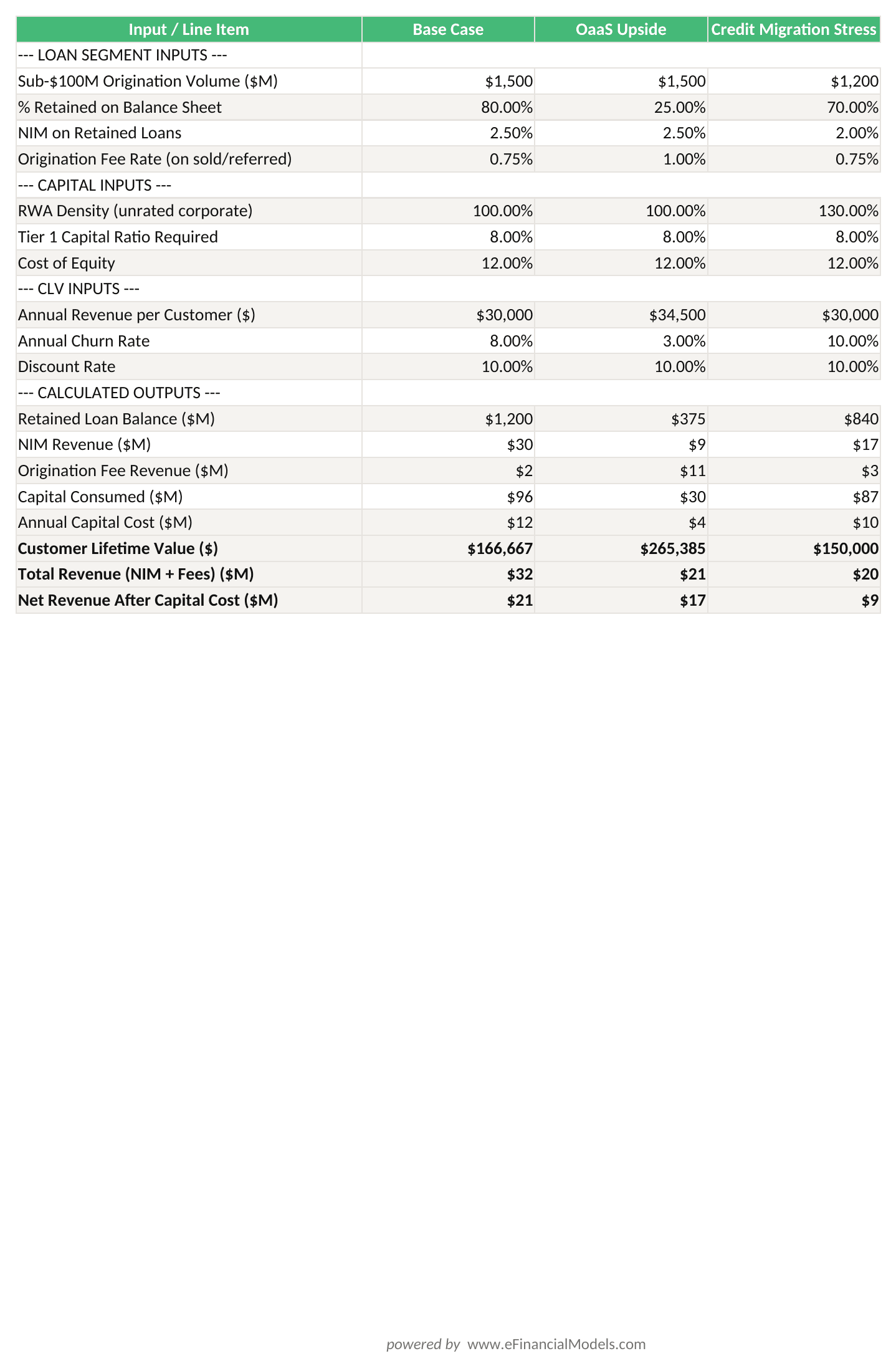
CLV (base) = $30,000 / (0.10 + 0.08) = $30,000 / 0.18 = $166,667
Now apply the precision model assumptions: 15% CLV improvement (midpoint of the 10-25% range) and a 5 percentage point reduction in churn from improved engagement:
- Adjusted annual revenue: $30,000 × 1.15 = $34,500
- Adjusted churn rate: 8% – 5% = 3%
- CLV (precision model) = $34,500 / (0.10 + 0.03) = $34,500 / 0.13 = $265,385
The precision model increases CLV by $98,718 per customer, a 59% improvement driven by both higher revenue and lower churn. Across a portfolio of 10,000 commercial customers, that is nearly $987 million in incremental relationship value. This number belongs in your strategic model as a quantified benefit of the precision engagement investment.

Risk Considerations: Credit Migration and Margin Compression Scenarios
Two risk factors are unique to the current banking environment and must appear explicitly in any credible bank cash-flow forecast: credit migration to non-banks and structural margin compression.
Credit migration risk occurs when the best-quality borrowers in the middle market refinance with non-bank lenders offering tighter spreads. The bank retains a progressively lower-quality loan book, which increases provision expense and reduces NIM simultaneously. Model this by building a credit quality migration matrix: each year, a percentage of investment-grade credits migrate to non-bank financing, and the bank’s retained portfolio shifts toward higher-risk, higher-spread (but higher-provision) exposures.
Margin compression is structural, not cyclical. As non-banks compete on price in the middle market, banks face a choice between matching spreads (compressing NIM) or losing volume (compressing fee income). Your model should include a margin compression scenario where NIM on retained middle-market loans declines 10-20 basis points annually over the five-year forecast period.
Regulatory capital scenario: Model a stress case where Basel III capital requirements tighten further, increasing the RWA density on unrated corporate exposures from 100% to 130%. This increases the capital cost per loan and further erodes return on equity for on-balance-sheet middle-market lending.

Implementation: Transitioning Your Bank Models to Reflect New Realities
Transitioning a legacy NIM-focused bank model to a modern strategic framework takes three phases. Each phase builds on the previous one and produces a usable model output at each stage.
Phase 1: Audit and Segment (Weeks 1-2)
Review your existing model’s revenue driver tree. Identify which loan segments are modeled as undifferentiated balance-sheet growth. Separate the loan book into the three competitive tiers described above. Flag any revenue line that does not distinguish between NIM income and fee income.
Phase 2: Rebuild Revenue Drivers (Weeks 3-5)
Replace the single NIM revenue line with a split model: retained loan NIM plus origination fee revenue. Add the RWA density and capital cost inputs for each segment. Build the CLV module with precision model scenario toggles. This phase typically requires the most time because it changes the fundamental logic of the model.
Phase 3: Integrate Risk and Scenario Framework (Weeks 6-8)
Add the credit migration matrix, margin compression assumptions, and Basel III stress scenarios. Build a scenario manager that lets users toggle between base case, origination-as-a-service upside, and credit migration downside. Validate the integrated model against the bank’s actual historical financials for at least two prior years before using it for forward projections.
For teams building this from scratch, a purpose-built bank financial model template provides the structural foundation and reduces Phase 2 build time significantly.
You can also explore financial forecasting models that incorporate scenario analysis frameworks directly applicable to the risk modeling phase described above.
For teams that need to present these projections to senior leadership, the pro forma income statement framework provides a clean output structure that integrates with the bank strategic model.
Frequently Asked Questions
What is the difference between a traditional bank cash-flow model and a modern strategic bank model?
A traditional bank cash-flow model projects revenue primarily as a function of loan balances multiplied by net interest margin. It treats the bank as the dominant lender in all segments and does not account for competitive displacement by non-bank lenders. A modern strategic bank model explicitly segments the loan book by competitive dynamics, separates NIM income from fee income, incorporates Basel III capital charges as a constraint on lending economics, and includes customer lifetime value as a revenue driver. The practical difference is significant: a traditional model might project 8% annual loan growth in the middle market, while a modern model would apply a 40-60% volume haircut to sub-$100M originations and replace that revenue with origination fee income. The two models produce materially different five-year cash-flow forecasts and lead to different strategic decisions about capital allocation.
How do I model origination-as-a-service fee revenue in a bank financial model?
Origination-as-a-service fee revenue is modeled as origination volume multiplied by fee rate. The key inputs are: total addressable origination volume in your target segment, the percentage of that volume the bank originates (origination market share), and the fee rate charged to the non-bank partner or investor who takes the loan onto their balance sheet. Typical fee rates run 0.5% to 1.5% of origination volume. For example, if your bank originates $1.5 billion in sub-$100M corporate loans annually and earns a 1% origination fee, the fee revenue line is $15 million. This revenue carries near-zero capital consumption, making the return on equity dramatically higher than holding the same loans on balance sheet at a 2.5% NIM with 100% RWA density.
What is Basel III and why does it matter for bank cash-flow forecasting?
Basel III is the international regulatory framework for bank capital adequacy, developed by the Basel Committee on Banking Supervision following the 2008 financial crisis. It requires banks to hold minimum levels of Tier 1 capital against risk-weighted assets. For corporate loans, the risk weight under the standardized approach is typically 100% for unrated borrowers, meaning a bank must hold roughly $8 in Tier 1 capital for every $100 lent. At a cost of equity of 12%, that is a $0.96 annual capital charge per $100 of exposure, before any credit loss provision. This capital cost is a structural disadvantage relative to non-bank lenders who face no equivalent requirement. In your cash-flow model, Basel III constraints should appear as explicit RWA density inputs and capital cost calculations for each loan segment, not as background assumptions.
How do I incorporate the McKinsey 20-30% engagement lift into a financial projection?
The 20-30 percentage point engagement lift from precision models translates into your model through the fee product penetration rate. Start with your current engagement rate, defined as the percentage of customers actively using three or more fee-generating products. Apply the engagement lift to that rate: if your current engagement rate is 35%, a 25 percentage point lift brings it to 60%. Then calculate the revenue impact: multiply the incremental engaged customers by the average annual fee revenue per engaged customer. If you have 50,000 commercial customers and the lift moves 12,500 additional customers into the engaged tier, and each engaged customer generates $8,000 more in annual fee revenue than a non-engaged customer, the revenue impact is $100 million annually. This becomes a scenario variable in your model, toggled on or off based on whether the bank has implemented precision engagement tools.
What is customer lifetime value (CLV) in banking and how is it calculated?
Customer lifetime value in banking is the present value of all future net revenue from a customer relationship. The standard formula for a steady-state relationship is: CLV = Annual Net Revenue / (Discount Rate + Annual Churn Rate). For a commercial banking customer generating $30,000 in annual net revenue with a 10% discount rate and 8% annual churn probability, CLV equals $30,000 divided by 0.18, or approximately $166,667. Precision engagement models improve CLV by increasing annual revenue per customer through higher product penetration and by reducing churn through stronger relationship depth. Applying the McKinsey 10-25% value improvement range to this base-case CLV produces an uplift of $16,667 to $41,667 per customer. Across a portfolio of thousands of commercial relationships, this improvement in CLV is a material strategic asset that belongs in any bank valuation or strategic planning model.
How should I model credit migration risk in a bank’s loan portfolio?
Credit migration risk in the current environment refers specifically to the risk that investment-grade or high-quality borrowers in the middle market refinance with non-bank lenders, leaving the bank with a progressively lower-quality retained portfolio. Model this using a migration matrix: assign each credit quality tier a probability of migrating to non-bank financing in each forecast year. For example, investment-grade sub-$100M borrowers might have a 15% annual migration probability, while below-investment-grade borrowers have a 5% migration probability (non-banks are less competitive for weaker credits). As investment-grade credits migrate out, the bank’s average provision rate on the retained portfolio rises, compressing net revenue even if total loan balances remain stable. A well-built model shows this dynamic explicitly rather than holding provision rates constant throughout the forecast period.
What discount rate should I use for a bank strategic cash-flow model?
For a bank strategic cash-flow model, the appropriate discount rate depends on what you are discounting. For equity cash flows to shareholders, use the cost of equity, typically estimated using the Capital Asset Pricing Model (CAPM). U.S. bank cost of equity has generally ranged from 9% to 13% in recent years, depending on the bank’s size, business mix, and systematic risk. For valuing specific business lines or fee revenue streams, use a segment-specific hurdle rate that reflects the risk of that cash flow: origination fee revenue is less capital-intensive and more predictable than NIM revenue, so it may warrant a slightly lower discount rate (8-10%) than on-balance-sheet lending returns (11-13%). Always document your discount rate assumptions explicitly in the model and run a sensitivity analysis showing how the strategic value changes across a 200-300 basis point range around your base-case rate.
Conclusion
Bank cash-flow forecasting has reached an inflection point. The combination of $2 trillion in private credit AUM, 60%+ non-bank origination share in the middle market, and Basel III capital constraints has made the traditional NIM-focused model structurally obsolete for strategic planning purposes. The banks that will generate superior returns over the next five years are those that model the shift to origination-as-a-service explicitly, quantify the CLV impact of precision engagement investments, and build credit migration risk into their base-case projections rather than their stress scenarios.
I recommend downloading a bank financial model template to get a pre-built framework that incorporates competitive segmentation, Basel III capital allocation, fee revenue projections, and customer lifetime value modeling. It gives your team a credible starting point for the Phase 2 rebuild described above and cuts weeks off the transition timeline.