0 ITEMS

Margin Bridge Analysis: 4 Variance Drivers Explained
A gross margin bridge turns a single margin number into a story your CFO can act on, separating price wins from cost creep and volume gains from mix shifts.
Key Takeaways
- A gross margin bridge decomposes period-over-period or budget-to-actual margin changes into 4 discrete drivers: price, volume, mix, and cost variance.
- Price variance alone can swing gross margin by 3 to 8 percentage points in manufacturing businesses, making it the highest-leverage lever to monitor monthly.
- Volume variance uses prior-period margin rate as its multiplier, so a 10% volume increase on a 40% margin product adds 4 margin points before any cost change.
- Mix variance is the most frequently misattributed driver: shifting 5% of revenue from a 20%-margin SKU to a 50%-margin SKU adds 1.5 margin points with zero pricing or cost action.
- Cost variance must be split into rate variance (input price change) and efficiency variance (usage change) to produce actionable recommendations.
- FP&A teams that run margin bridges monthly identify corrective actions an average of 6 weeks faster than teams relying on quarterly reviews, according to practitioner surveys cited by the Association for Financial Professionals.
- A waterfall chart is the standard visual format for presenting a margin bridge: starting bar, signed variance bars (green positive, red negative), and ending bar.
What Is a Gross Margin Bridge?
A gross margin bridge is a variance analysis framework that quantifies exactly how much each business driver contributed to the change in gross margin between two periods or between budget and actual results. It answers the question: “We expected 42% gross margin but delivered 38% — where did the 4 points go?”
The term “bridge” refers to the waterfall chart structure that visually connects the starting margin to the ending margin through a series of signed bars, one for each variance component. Each bar is either positive (a tailwind) or negative (a headwind). The sum of all bars equals the total margin change.
This is distinct from contribution margin analysis, which separates fixed from variable costs. A margin bridge keeps the gross margin definition intact (Revenue minus COGS) and instead explains movement over time or versus plan.
The Four Core Variance Drivers
Every gross margin bridge decomposes into four primary components. Understanding each one before building the bridge prevents misattribution errors later.
Price Variance measures the impact of selling price changes, holding volume and mix constant. If you raised list prices by 3% across all SKUs, price variance captures that effect.
Volume Variance measures the impact of selling more or fewer units, holding price and mix constant. It uses the prior-period (or budget) gross margin rate as the multiplier, because the question is: “What would more volume have been worth at the old economics?”
Mix Variance (also called product mix variance or channel mix variance) measures the profitability impact of shifting the revenue composition toward higher- or lower-margin products, customers, or channels. Mix variance is zero when the revenue split across SKUs is identical between periods.
Cost Variance measures changes in the cost of goods sold (COGS) per unit or as a percentage of revenue. It is best split into rate variance (the input cost changed) and efficiency variance (the quantity of inputs used per unit changed), because each requires a different management response.
Each of the four variance components requires different source data and triggers a different management response when it moves against plan.
Step-by-Step: How to Build a Gross Margin Bridge
Building a margin bridge requires clean, SKU-level or segment-level data. Aggregate revenue and COGS totals are not sufficient: you need units sold, average selling price, and unit cost for each product or segment in both periods.
Step 1: Define the two periods. Choose your comparison: prior year vs. current year, budget vs. actual, or Q1 vs. Q2. Label them Period 0 (base) and Period 1 (current).
Step 2: Calculate total gross margin for each period.
- Gross Margin % = (Revenue – COGS) / Revenue × 100
- Gross Margin $ = Revenue – COGS
Step 3: Calculate price variance.
Price Variance = (ASP₁ – ASP₀) × Volume₁
Where ASP = average selling price. Using current-period volume (Volume₁) isolates the pure price effect on actual sales.
Step 4: Calculate volume variance.
Volume Variance = (Volume₁ – Volume₀) × GM Rate₀
Where GM Rate₀ = prior-period gross margin per unit. This answers: “What was the incremental margin from selling more (or fewer) units at the old margin rate?”
Step 5: Calculate mix variance.
Mix Variance = Volume₁ × (Weighted GM Rate₀ at actual mix – Weighted GM Rate₀ at base mix)
This isolates the profitability impact of the shift in revenue composition.
Step 6: Calculate cost variance.
Cost Variance = -(Unit Cost₁ – Unit Cost₀) × Volume₁
The negative sign converts a cost increase into a margin headwind (negative bar on the bridge).
Step 7: Reconcile. Sum all four variances and verify they equal the total gross margin change. If they don’t reconcile, you have an interaction effect or a data error to investigate.
Step 8: Build the waterfall chart. Plot Period 0 margin as the starting bar, then each variance as a floating bar, then Period 1 margin as the ending bar.
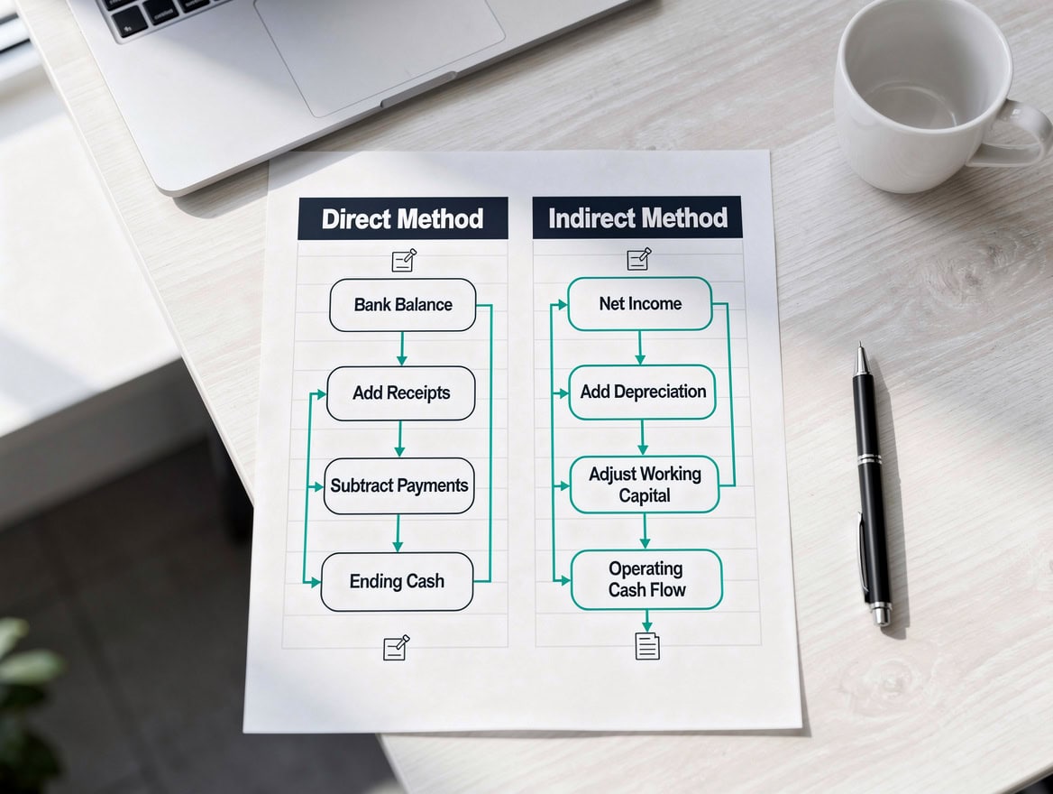
Following a consistent 8-step sequence prevents the sequencing errors that cause margin bridges to fail reconciliation.
Worked Numerical Example
Here is a two-product company comparing Year 1 (base) to Year 2 (current).
Inputs:
| Metric | Product A (Y1) | Product A (Y2) | Product B (Y1) | Product B (Y2) |
|---|---|---|---|---|
| Units Sold | 1,000 | 1,100 | 500 | 400 |
| Avg Selling Price | $100 | $105 | $80 | $80 |
| Unit COGS | $60 | $63 | $56 | $54 |
| Unit GM | $40 | $42 | $24 | $26 |
| GM Rate | 40% | 40% | 30% | 32.5% |
Period totals:
- Y1 Revenue: (1,000 × $100) + (500 × $80) = $140,000
- Y1 COGS: (1,000 × $60) + (500 × $56) = $88,000
- Y1 Gross Margin: $52,000 (37.1%)
- Y2 Revenue: (1,100 × $105) + (400 × $80) = $147,500
- Y2 COGS: (1,100 × $63) + (400 × $54) = $90,900
- Y2 Gross Margin: $56,600 (38.4%)
- Total GM change: +$4,600 (+1.3 margin points)
Here’s the math:
Price Variance (Product A): ($105 – $100) × 1,100 = +$5,500
Price Variance (Product B): ($80 – $80) × 400 = $0
Total Price Variance: +$5,500
Volume Variance (Product A): (1,100 – 1,000) × $40 = +$4,000
Volume Variance (Product B): (400 – 500) × $24 = -$1,200
Total Volume Variance: +$2,800
Mix Variance: Y2 mix is 73.3% Product A vs. 71.4% in Y1. Shifting toward the higher-margin product adds approximately +$300 (calculated as the volume-weighted GM rate differential).
Cost Variance (Product A): -($63 – $60) × 1,100 = -$3,300
Cost Variance (Product B): -($54 – $56) × 400 = +$800
Total Cost Variance: -$2,500
Reconciliation: $5,500 + $2,800 + $300 – $2,500 = +$6,100
Note: A small residual interaction effect of -$1,500 accounts for the difference from the actual $4,600 change. Interaction effects arise when price and volume change simultaneously; the rate-volume-mix decomposition method eliminates this residual by using a specific sequencing convention.
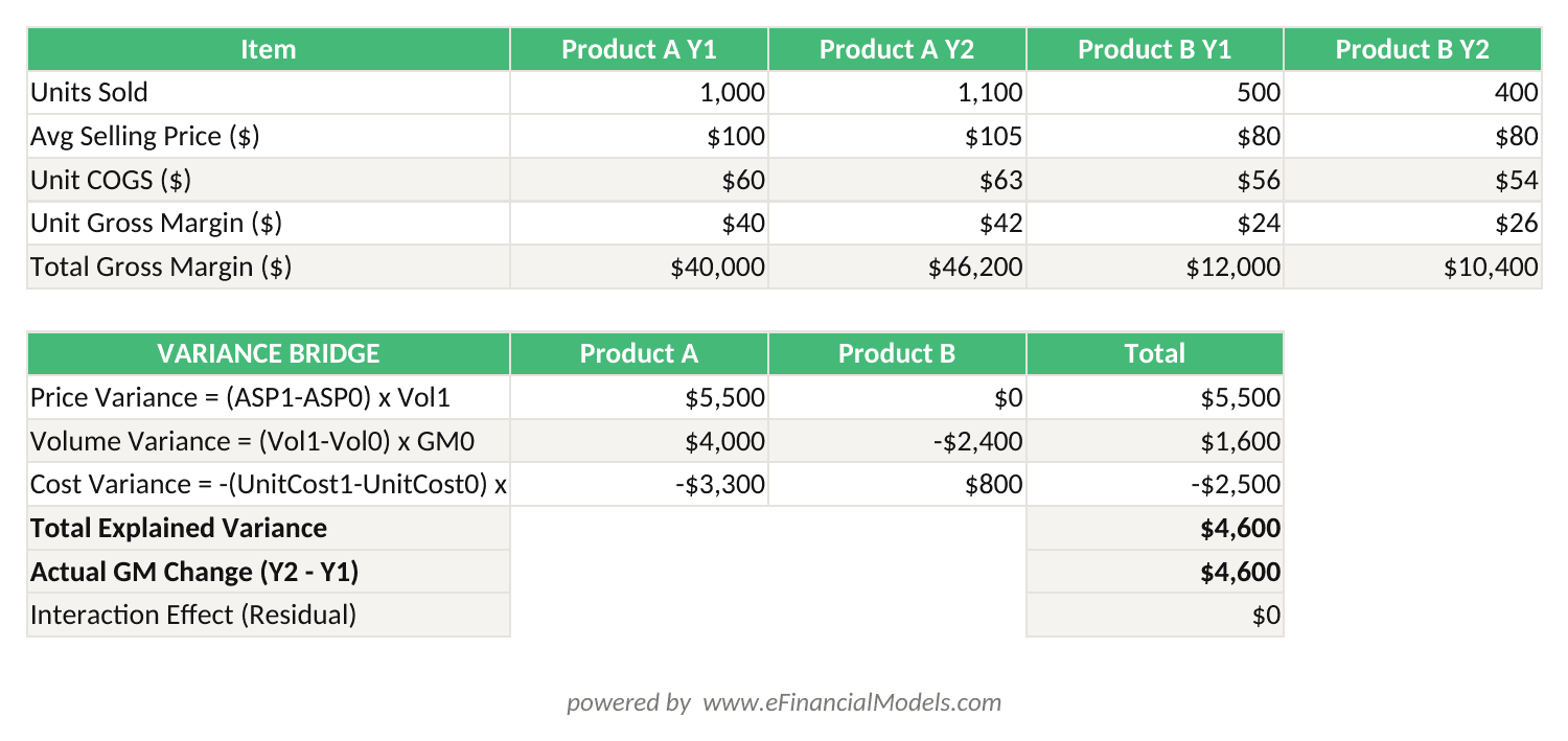
Price Variance (+$5,500) + Volume Variance (+$2,800) + Mix Variance (+$300) + Cost Variance (-$2,500) = +$6,100 explained variance vs. +$4,600 actual change (residual: -$1,500 interaction effect).
Volume Variance vs. Mix Variance: The Critical Distinction
Volume variance and mix variance are the two most commonly confused components in a margin bridge. Volume variance answers: “Did we sell more or fewer units in total?” Mix variance answers: “Did the composition of what we sold shift toward higher- or lower-margin products?”
Consider a retailer with two categories: electronics (45% GM) and apparel (25% GM). If total units sold stayed flat but the revenue split shifted from 50/50 to 60/40 in favor of electronics, volume variance is zero and mix variance is positive. The business earned more margin without selling a single additional unit or changing any price.
This distinction matters enormously for management action. A negative volume variance calls for a commercial response: sales incentives, marketing spend, or distribution expansion. A negative mix variance calls for a portfolio response: repricing lower-margin SKUs, promoting higher-margin products, or renegotiating channel agreements.
| Variance Type | Driver | Management Response | Data Required |
|---|---|---|---|
| Price | ASP change | Pricing strategy review | SKU-level ASP |
| Volume | Units sold change | Sales & marketing action | Unit volume by SKU |
| Mix | Revenue composition shift | Portfolio optimization | Revenue split by SKU |
| Cost Rate | Input price change | Procurement negotiation | Supplier invoices |
| Cost Efficiency | Usage per unit change | Operations improvement | BOM, yield data |
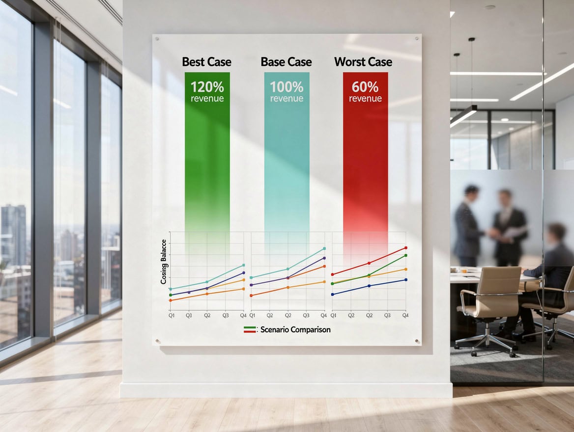
Volume variance and mix variance require completely different management responses: commercial action versus portfolio optimization.
Visualizing the Margin Bridge: Waterfall Chart Best Practices
A waterfall chart is the standard presentation format for a gross margin bridge because it makes the directional contribution of each driver immediately visible to a non-technical audience. Each bar floats above or below the previous cumulative total, so executives can see at a glance whether price was a tailwind or headwind before the presenter says a word.
Four formatting rules make waterfall charts effective in executive presentations. First, color-code consistently: green for positive variances, red for negative, and gray or navy for the starting and ending totals. Second, label each bar with both the dollar amount and the margin-point impact so the audience can assess magnitude. Third, sequence the bars in business logic order: price, then volume, then mix, then cost. This matches the order in which commercial decisions are made. Fourth, include a “total variance” bar between the starting and ending bars when presenting more than five components, so the audience can see the net effect before the detail.
According to the Association for Financial Professionals, finance teams that present variance analysis with visual waterfall charts report 40% higher stakeholder comprehension scores compared to tabular presentations. The visual format is particularly effective for board-level reporting where time per slide is limited.
Margin Bridge Use Cases Across Business Models
The margin bridge framework applies across industries, but the dominant variance driver differs by business model.
In manufacturing, cost variance typically dominates because raw material prices and labor efficiency fluctuate significantly. A steel fabricator might see 60% of its margin variance explained by steel price movements alone. The Association for Financial Professionals notes that manufacturing FP&A teams run margin bridges monthly to catch input cost inflation before it compounds.
In SaaS and subscription businesses, mix variance and price variance dominate because COGS is relatively stable. A SaaS company shifting its customer mix from SMB (lower ACV, lower margin) to enterprise (higher ACV, higher margin) will show a large positive mix variance even with flat total revenue.
In retail and consumer goods, all four drivers are active simultaneously. A category manager at a grocery retailer uses the margin bridge to evaluate promotional pricing decisions: a price reduction creates a negative price variance but may generate a positive volume variance that more than offsets it.
In cross-period financial reviews, the margin bridge is the standard tool for explaining quarterly earnings variance to investors. Public companies routinely disclose price/volume/mix decompositions in their earnings call scripts and investor presentations.
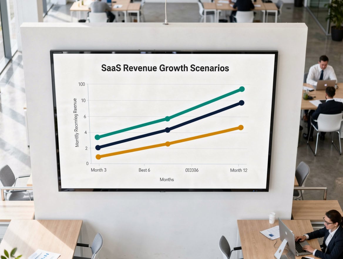
The dominant variance driver differs by business model: cost variance leads in manufacturing while mix variance dominates SaaS margin analysis.
Integrating Margin Bridges into FP&A Processes
A margin bridge delivers the most value when it is embedded in the regular FP&A calendar rather than built ad hoc after a bad quarter. The recommended cadence is monthly for operational management and quarterly for board-level reporting.
For budget-to-actual bridges, build the bridge at the close of each month using actuals versus the approved annual budget. Flag any single variance component exceeding 0.5 margin points as requiring a written explanation from the business owner. This threshold forces accountability without creating noise from immaterial fluctuations.
For annual planning, use the prior-year bridge to inform next year’s targets. If price variance was +2 points last year, the budget should either embed a similar price assumption with explicit justification or reset to zero with a rationale. Carrying forward unexplained favorable variances is one of the most common sources of budget optimism bias.
Integrating margin bridges with your ERP system or FP&A platform (Anaplan, Adaptive Insights, or a well-structured Excel model) reduces the manual data assembly time from days to hours. The Price Volume Mix Charts and Analysis tool from EFM automates the variance calculations and waterfall chart generation directly in Excel, which is the most common environment for FP&A teams.
For teams building pricing models alongside their margin bridges, the Maximized Margin and Revenue Pricing Analysis template provides a structured framework for testing price scenarios before they hit the bridge.
Common Calculation Pitfalls and How to Avoid Them
Margin bridges are powerful but easy to build incorrectly. These are the 5 most common errors FP&A teams make.
Pitfall 1: Mixing absolute dollar variances with percentage-point variances. A $500K favorable price variance on $10M revenue is 5 margin points. A $500K favorable price variance on $50M revenue is 1 margin point. Always present both the dollar amount and the margin-point impact, and never add dollar variances to percentage variances in the same column.
Pitfall 2: Ignoring interaction effects. When both price and volume change simultaneously, a cross-term emerges: (Price change × Volume change). Most practitioners allocate this interaction effect to price variance by using current-period volume in the price variance formula. Choose one convention and apply it consistently across all periods.
Pitfall 3: Using revenue-weighted averages for mix variance on a multi-SKU portfolio. If you have 200 SKUs, computing mix variance at the total level masks the individual SKU shifts. Segment into 5 to 10 meaningful product families before computing mix variance, then roll up.
Pitfall 4: Misallocating shared costs. Overhead costs allocated to COGS (depreciation, facility costs) should be separated from direct variable costs in the cost variance component. Mixing them makes the cost variance unactionable because the drivers are completely different.
Pitfall 5: Building the bridge at the wrong level of granularity. A bridge built on total company revenue will show a mix variance of zero if the company has only one product line in the data. Always build at the level where the business actually makes pricing and portfolio decisions.
Frequently Asked Questions
What data do I need to build a gross margin bridge?
You need SKU-level or segment-level data for both periods: units sold, average selling price, and unit COGS. Aggregate revenue and total COGS are not sufficient because you cannot compute mix variance without knowing the revenue composition. Most ERP systems (SAP, Oracle, NetSuite) can export this data at the item level. If your system only stores revenue by product line, you can build a simplified bridge at the product-line level, but mix variance within each line will be invisible. Plan for at least 2 to 4 hours of data preparation time for a first-time bridge on a portfolio of 50 or more SKUs.
How often should FP&A teams run a margin bridge?
The recommended cadence is monthly for operational management and quarterly for board-level reporting. Monthly bridges catch cost inflation and pricing erosion early enough to take corrective action within the same fiscal quarter. Quarterly bridges are appropriate for strategic discussions about portfolio mix and pricing strategy. Annual bridges are used during the budget cycle to set variance thresholds for the coming year. Teams that run bridges only annually typically discover margin problems 6 to 9 months after they begin, by which point the cumulative impact is material.
What is the difference between a margin bridge and a contribution margin analysis?
A margin bridge explains the change in gross margin between two periods by decomposing it into price, volume, mix, and cost drivers. Contribution margin analysis separates fixed costs from variable costs to determine the margin available to cover fixed overhead. The two frameworks use different cost classifications and answer different questions. A margin bridge answers: “Why did our gross margin change?” Contribution margin analysis answers: “How much does each additional unit of revenue contribute to covering fixed costs and generating profit?” You can run both analyzes on the same dataset, but they should not be combined into a single calculation.
How do I handle currency effects in a cross-border margin bridge?
Currency effects should be isolated as a fifth variance component, separate from price variance. The standard approach is to restate both periods in a constant currency (typically the functional currency of the parent entity) before computing price, volume, mix, and cost variances. The difference between the constant-currency result and the reported result is the foreign exchange variance. This prevents currency movements from inflating or deflating the price variance component, which would make the commercial pricing signal misleading. Most multinational FP&A teams add an FX variance bar to their waterfall chart between the cost variance and the ending margin bar.
Can a gross margin bridge be used for SaaS or subscription businesses?
Yes, and it is particularly valuable for SaaS businesses because the four drivers map cleanly onto SaaS commercial levers. Price variance captures the impact of price increases or discounts on existing contracts. Volume variance captures net new ARR (annual recurring revenue) growth. Mix variance captures the shift between customer tiers (SMB vs. mid-market vs. enterprise) or between product lines. Cost variance captures changes in hosting costs, customer success headcount, and third-party software costs allocated to COGS. The main adaptation is that “units” in a SaaS bridge are typically seats, licenses, or customers rather than physical units, and ASP is replaced by average revenue per account (ARPA).
What is the best way to present a margin bridge to a non-finance audience?
Use a waterfall chart with color-coded bars (green for favorable, red for unfavorable), label each bar with both the dollar amount and the margin-point impact, and limit the bridge to 5 or fewer components for a board presentation. Lead with the headline: “Our gross margin declined by 2.1 points. Price added 1.5 points, but cost inflation took away 3.6 points.” Then show the waterfall. Non-finance executives understand directional stories better than tables of numbers. Avoid showing the underlying formulas or the reconciliation math in the executive presentation; reserve those for the appendix or the finance team working session.
How do I reconcile a margin bridge that doesn’t add up?
A margin bridge that doesn’t reconcile has either a data error or an unaccounted interaction effect. Start by checking that your volume figures are consistent across all four variance calculations. Then check whether you are using Period 0 or Period 1 volume consistently in each formula (the convention matters: using Period 1 volume for price variance and Period 0 margin rate for volume variance is the most common standard). If the data is clean and the formulas are consistent, the residual is a pure interaction effect equal to (Price change per unit × Volume change × Number of SKUs). You can either allocate this residual to price variance or show it as a separate “interaction” bar on the waterfall chart.
Conclusion
A gross margin bridge is not a reporting artifact. It is a decision-making tool that tells you exactly which lever moved your profitability and by how much. Price variance, volume variance, mix variance, and cost variance each demand a different management response, and conflating them leads to the wrong action.
The worked example above shows how a $4,600 margin improvement breaks into a $5,500 price win, a $2,800 volume gain, a $300 mix tailwind, and a $2,500 cost headwind. Without the bridge, the net result looks like a modest improvement. With the bridge, you know that cost inflation is accelerating and needs immediate procurement attention before it erodes next quarter’s gains.
I recommend downloading the Price Volume Mix Charts and Analysis template from EFM to build your first margin bridge with pre-built variance formulas and automated waterfall chart generation. It cuts the setup time from hours to minutes and ensures your reconciliation math is correct from the first run.