0 ITEMS

Gold Mine Scenario Analysis: AUD/USD and Grade Risk

Gold mine scenario analysis is the practice of recalculating a mine’s value under several internally consistent combinations of price, exchange rate, and ore grade, rather than relying on a single base case. For an Australian gold project, the two variables that move value most are the AUD/USD exchange rate, because revenue is earned in US dollars while costs are paid in Australian dollars, and the head grade fed to the mill, because grade drives both ounces produced and all-in sustaining cost per ounce. Done well, scenario analysis turns a fragile point estimate into a probability-weighted range a lender or investment committee can actually trust.
Key Takeaways
- Gold mine scenario analysis recalculates net present value across linked price, AUD/USD, and grade cases, not one variable at a time.
- Australian gold revenue is priced in US dollars while most costs are in Australian dollars, so a move in AUD/USD from 0.72 to 0.62 can lift the Australian-dollar gold price received by more than 16%.
- Global gold all-in sustaining cost has climbed to record highs near US$1,600 per ounce, so margin, not just headline price, decides which projects survive a downturn.
- A 20% drop in head grade typically raises all-in sustaining cost per ounce by a similar magnitude, because fixed mining and processing costs are spread over fewer recovered ounces.
- The eFinancialModels Australia Mining Market Study 2026-2031 weights its outlook 25% bear, 50% base, and 25% bull, a structure you can copy directly into a project model.
- A worked three-case model below shows annual margin swinging from A$89 million to A$534 million on the same 150,000-ounce mine.
What Is Gold Mine Scenario Analysis?
Gold mine scenario analysis is a valuation technique that runs a project model through several complete, plausible states of the world and reports the resulting spread in net present value (NPV) and internal rate of return (IRR). NPV is the present value of future cash flows minus upfront investment, and IRR is the discount rate at which NPV equals zero. Each scenario fixes a coherent set of assumptions, for example a weak gold price paired with a strong Australian dollar and a low realised grade, so the model captures how risks combine rather than how they behave in isolation.
Scenario analysis versus sensitivity analysis
Scenario analysis and sensitivity analysis answer different questions, and a strong model uses both. Sensitivity analysis flexes one input at a time, such as the gold price, to measure how steeply value responds to that single lever. Scenario analysis instead bundles several inputs into named cases, because in the real world a falling gold price often arrives alongside a flight to the US dollar and tighter mine plans. The eFinancialModels scenario analysis and sensitivity analysis template tags collect models built for exactly this distinction.
Why gold mines need both
Gold projects need both methods because their cash flows are leveraged to small percentage moves in price, currency, and grade. A mine running close to its all-in sustaining cost can flip from strongly profitable to loss making on a modest combination of adverse moves, which a single base case hides. Sensitivity analysis tells you which input to watch, and scenario analysis tells you what happens when the worst of them line up. For a consultant signing off a model, presenting both is the difference between a defensible recommendation and an optimistic guess.
Why AUD/USD Drives Australian Gold Mine Returns
The AUD/USD exchange rate drives Australian gold returns because gold is sold in US dollars while wages, fuel, power, and royalties are paid in Australian dollars. When the Australian dollar weakens against the US dollar, every US-dollar ounce converts into more Australian dollars, expanding the local-currency margin without any change in the gold price itself. As at 26 June 2026 the Reserve Bank of Australia recorded the Australian dollar near 0.69 US cents (Reserve Bank of Australia), a level that has swung several cents within a single year.
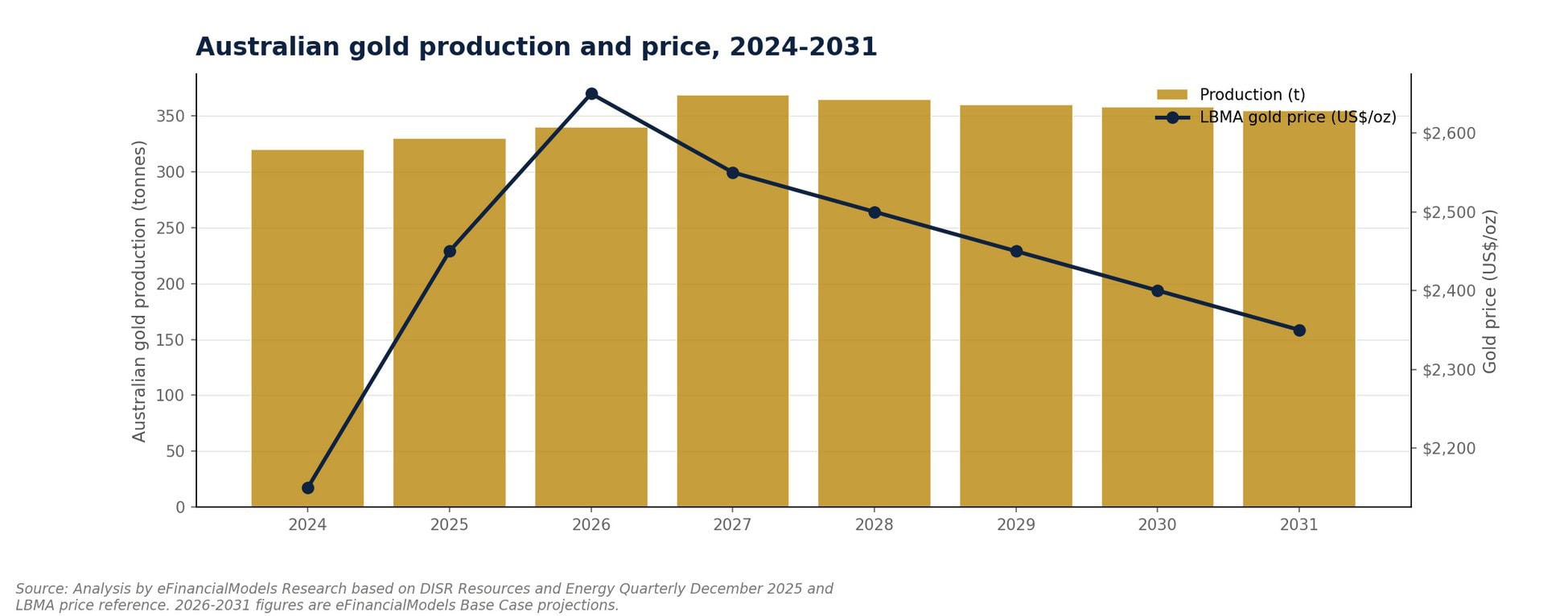
Australian gold output is forecast to rise even as the modeled US-dollar price eases, which makes the AUD/USD rate the swing factor for local margins. Source: eFinancialModels Australia Mining Market Study 2026-2031.
The two-currency problem
The two-currency problem is the structural mismatch between US-dollar revenue and Australian-dollar costs that sits at the heart of every Australian gold model. A miner cannot control the US-dollar gold price or the exchange rate, yet both feed the same revenue line, so currency risk and commodity risk are entangled. The London Bullion Market Association gold price set a record quarterly average near US$4,873 per ounce in the first quarter of 2026 (World Gold Council), and a weaker Australian dollar amplified that strength for domestic producers. Modelers who hardcode a single exchange rate quietly assume away one of the two largest sources of variance.
Modeling the exchange rate in your cash flow
Model AUD/USD as an explicit input feeding the revenue conversion, never as a number buried inside the gold price assumption. The cleanest structure holds the US-dollar gold price and the AUD/USD rate as separate cells, then derives the Australian-dollar price received as the US-dollar price divided by the rate. This keeps the two-currency problem visible and lets you scenario the rate independently of the metal price. It also matches how Australian resource and energy export earnings are reported, which the government forecasts at A$383 billion for 2025-26 (Department of Industry, Science and Resources).
How Ore Grade Sensitivity Changes the Model
Ore grade sensitivity changes the model because grade controls both the numerator and the denominator of unit economics: more grade means more recovered ounces over the same tonnes mined, and lower cost spread across each of those ounces. Head grade is the concentration of gold in the ore fed to the processing plant, usually quoted in grams per tonne. Small changes in head grade move output and all-in sustaining cost in opposite, reinforcing directions, which is why grade deserves its own scenario axis alongside price and currency.
Head grade and the grade-tonnage relationship
Head grade and the grade-tonnage curve together set how many payable ounces a deposit yields. The grade-tonnage relationship describes how available tonnes change as the cut-off grade, the minimum grade worth processing, is raised or lowered. Drop the cut-off to chase tonnes and average grade falls, lifting cost per ounce; raise it to protect grade and the mine life shortens. A scenario model should therefore link grade to both the production schedule and the cost base, not treat it as a standalone revenue tweak.
Grade’s leverage on AISC and NPV
Grade exerts outsized leverage on all-in sustaining cost (AISC), the cash cost of producing an ounce plus sustaining capital and overhead. Because a large share of mining and milling cost is fixed per tonne rather than per ounce, fewer ounces from lower grade spread those costs thinly, pushing AISC up. With global gold AISC already at record highs near US$1,600 per ounce (World Gold Council), a grade-driven cost rise can erase the margin that price strength provides. In the worked model below, a 20% grade reduction lifts AISC by roughly 20% and cuts annual margin sharply, even before any adverse price or currency move.
How to Build a Gold Mine Scenario Matrix in 5 Steps

Build the matrix by defining cases first, then letting linked formulas compute every output, so the model recalculates instantly when an assumption changes. The five steps below produce a bear, base, and bull view that mirrors the structure used in the eFinancialModels Australia Mining Market Study 2026-2031.
- Set the shared engine. Build one cash flow that converts a US-dollar gold price at an explicit AUD/USD rate, applies a grade factor to AISC, and multiplies margin per ounce by annual ounces.
- Define three coherent cases. Pair each gold price with an exchange rate and a grade that belong together, for example low price with a strong Australian dollar and low grade for the bear case.
- Assign probabilities. Weight the cases, for example 25% bear, 50% base, and 25% bull, so the output is a probability-weighted expected value rather than three disconnected numbers.
- Compute margin and NPV per case. Calculate Australian-dollar margin per ounce and annual margin for each scenario, then discount multi-year cash flows to NPV using a consistent rate.
- Report the range and the drivers. Present the spread, the weighted expectation, and which variable moved value most, so the committee sees both the downside and its cause.
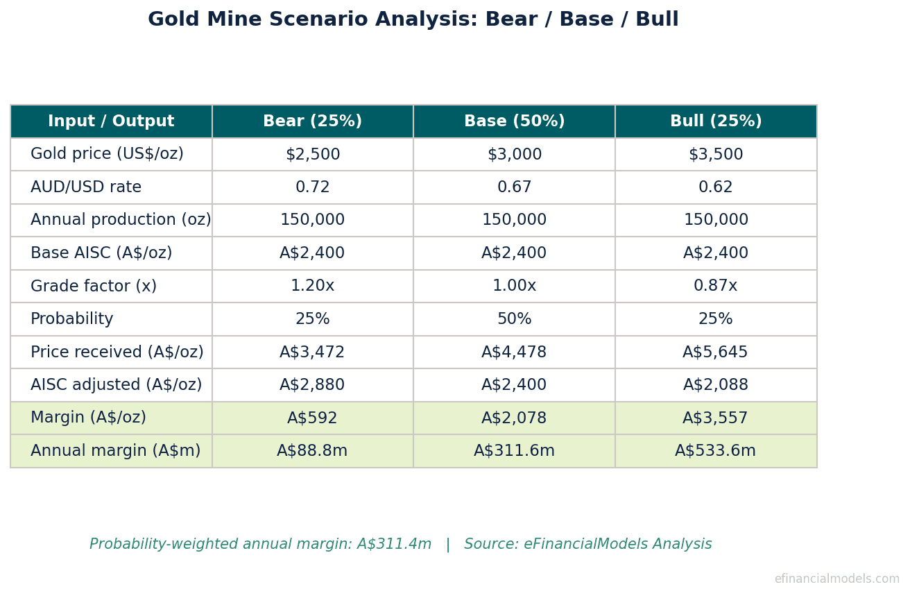
Worked three-case gold mine scenario model with formula-driven outputs. Source: eFinancialModels Analysis.
Gold Mine Scenario Analysis Example: Bear, Base, Bull
A worked example makes the leverage concrete. The model below takes a single Australian open-pit mine producing 150,000 ounces a year and runs it through three linked cases, converting a US-dollar gold price at an explicit AUD/USD rate and adjusting AISC for grade. Each Australian-dollar price received equals the US-dollar price divided by the exchange rate, and annual margin equals margin per ounce multiplied by annual ounces.
| Input / Output | Bear (25%) | Base (50%) | Bull (25%) |
|---|---|---|---|
| Gold price (US$/oz) | 2,500 | 3,000 | 3,500 |
| AUD/USD rate | 0.72 | 0.67 | 0.62 |
| Price received (A$/oz) | 3,472 | 4,478 | 5,645 |
| Grade factor on AISC | 1.20 (low grade) | 1.00 | 0.87 (high grade) |
| AISC (A$/oz) | 2,880 | 2,400 | 2,088 |
| Margin (A$/oz) | 592 | 2,078 | 3,557 |
| Annual margin (A$m) | 88.8 | 311.6 | 533.6 |
The probability-weighted annual margin is about A$311 million, close to the base case, but the range from A$89 million to A$534 million is the real story. The bear column shows how a strong Australian dollar, a soft gold price, and a low realised grade combine to compress margin by more than 70% against base, even though no single input collapses. That combined downside is invisible to a one-variable sensitivity test, which is precisely why a gold mine scenario analysis matters.
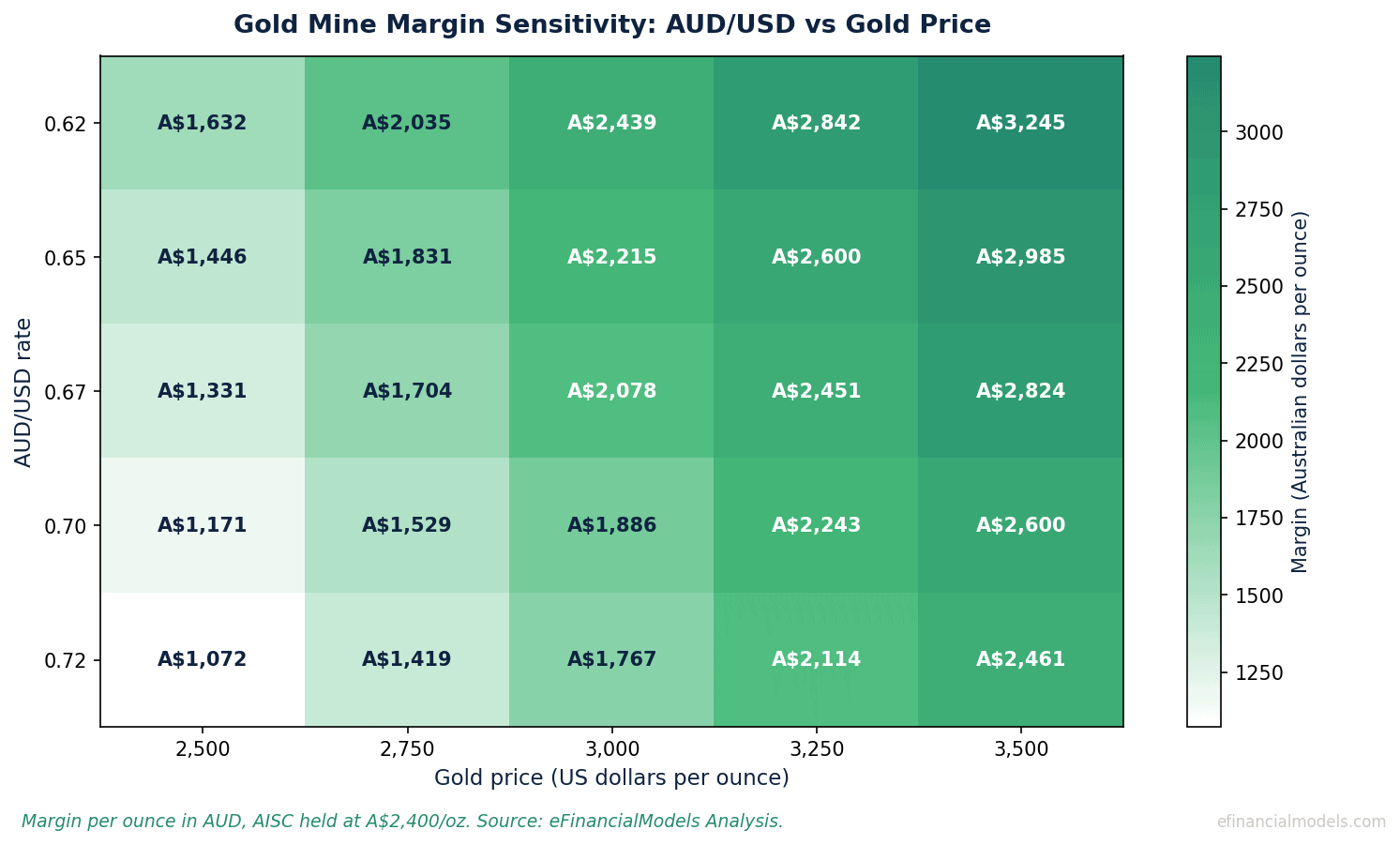
Margin per ounce sensitivity to AUD/USD and the US dollar gold price. Source: eFinancialModels Analysis.
Common Mistakes in Gold Mine Scenario Analysis
The most common mistake is treating the exchange rate, gold price, and grade as independent when building cases. Avoiding a handful of recurring errors keeps a scenario model honest and credible.
- Burying AUD/USD inside the gold price. Keep the rate as its own input so currency risk can be scenarioed and audited separately from metal price.
- Holding AISC flat across grades. Lower grade should raise AISC per ounce in the model, because fixed costs spread over fewer ounces; a flat AISC overstates the downside protection.
- Mixing optimistic inputs across cases. A credible bear case pairs adverse moves together rather than cherry-picking a low price with an unrealistically weak Australian dollar that would actually help.
- Ignoring probabilities. Three unweighted cases describe a range but give no expected value; assigning weights such as 25/50/25 produces a number a committee can act on.
- Using spot instead of a planning price. Spot gold near US$4,000 per ounce in mid-2026 flatters every case; through-cycle planning prices keep the analysis defensible across the mine life.
Frequently Asked Questions
What is gold mine scenario analysis?
Gold mine scenario analysis is a valuation method that recalculates a mine’s net present value and internal rate of return across several internally consistent cases, each combining a gold price, an exchange rate, and an ore grade. Unlike a single base case, it shows the full range of outcomes and a probability-weighted expectation. For Australian gold projects the most important axes are AUD/USD and head grade, because they drive both revenue conversion and all-in sustaining cost. A typical structure uses three cases, bear, base, and bull, weighted by probability.
How does the AUD/USD exchange rate affect a gold mine model?
The AUD/USD exchange rate affects the model because gold is sold in US dollars while Australian mines pay costs in Australian dollars. When the Australian dollar weakens, each US-dollar ounce converts into more Australian dollars, lifting local-currency margin with no change in the metal price. In the worked example above, moving from 0.72 to 0.62 raises the Australian-dollar price received from A$3,472 to A$5,645 per ounce on a US$2,500 to US$3,500 price range. The Reserve Bank of Australia recorded the rate near 0.69 in late June 2026.
How does ore grade sensitivity change all-in sustaining cost?
Ore grade sensitivity changes all-in sustaining cost because a large share of mining and processing cost is fixed per tonne, so fewer ounces from lower grade spread those costs across a smaller base. A roughly 20% reduction in head grade tends to raise AISC per ounce by a similar magnitude. With global gold AISC at record highs near US$1,600 per ounce, grade-driven cost increases can wipe out margin that a higher gold price would otherwise deliver. That is why grade belongs on its own scenario axis rather than as a simple revenue adjustment.
What probabilities should I assign to bear, base, and bull cases?
A common and defensible starting point is 25% bear, 50% base, and 25% bull, the same weighting used in the eFinancialModels Australia Mining Market Study 2026-2031. These weights place the most confidence in the central case while giving meaningful mass to both tails, producing a probability-weighted expected value rather than three disconnected numbers. You should adjust the weights to reflect deposit-specific risk, hedging, and the maturity of the project. Document the rationale so reviewers can challenge the weighting rather than guess at it.
What is the difference between scenario analysis and sensitivity analysis?
Sensitivity analysis flexes one input at a time to measure how steeply value responds to that single variable, while scenario analysis bundles several inputs into coherent cases that move together. A gold mine model needs both: sensitivity analysis identifies which lever matters most, and scenario analysis shows what happens when adverse moves combine. Relying on sensitivity alone hides correlated risk, such as a falling gold price arriving with a flight to the US dollar. Presenting both gives a far more complete picture of project risk.
Which financial model template is best for gold mine scenario analysis?
The best template is one that already separates US-dollar price, exchange rate, grade, and AISC as distinct inputs feeding a single cash flow engine. The eFinancialModels mining and resources model library includes gold-focused templates, such as project-finance and DCF valuation models, with scenario and sensitivity tables built in. Choosing a ready template saves the days of structuring work that scenario analysis otherwise requires and reduces the risk of formula errors. Look specifically for an explicit AUD/USD cell and a grade-linked AISC, the two features this article shows to matter most.
Conclusion: Model the Combination, Not Just the Price
Gold mine scenario analysis earns its keep when it captures how AUD/USD and ore grade move together, because that combination, not the headline gold price alone, decides whether an Australian project clears its cost of capital. Build the exchange rate and a grade-linked AISC as explicit inputs, weight your bear, base, and bull cases, and report the range alongside the expectation. I recommend pairing the Australia Mining Market Study 2026-2031 with a ready template from the eFinancialModels gold and mining model library, which give you the two-currency engine and scenario structure ready to populate with your own deposit data.