0 ITEMS

Discounted Cash Flow Model: A Step-by-Step Excel Walkthrough

A discounted cash flow (DCF) model values a business by forecasting its free cash flow and discounting those cash flows back to today at a rate that reflects risk. This guide builds one in five steps from Procter & Gamble’s fiscal 2026 annual report, then shows the mistakes that most often distort the result.
Key Takeaways
- A DCF model has five steps: forecast free cash flow, build the discount rate, add terminal value, subtract net debt, then stress the result.
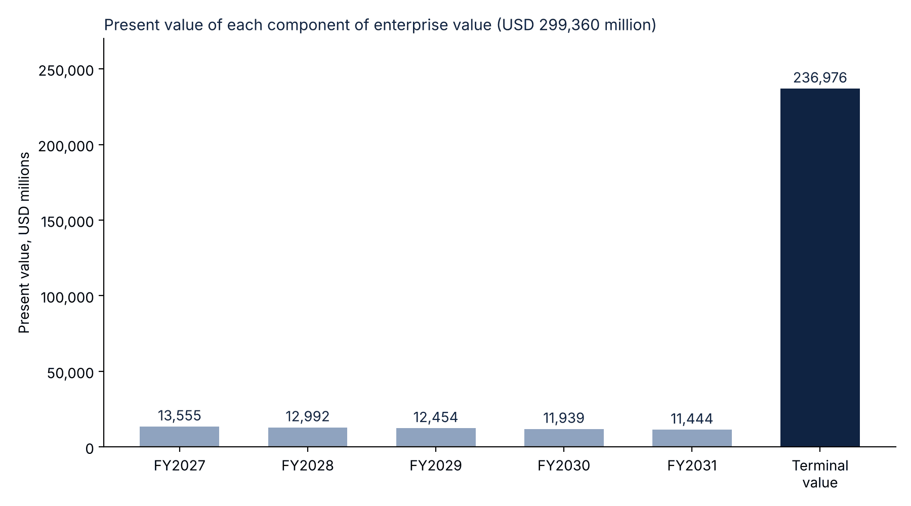
- Terminal value supplies 79.2% of enterprise value in the worked example, so the terminal growth rate and discount rate drive the answer.
- Terminal growth cannot exceed the growth rate of the overall economy; the example uses 2.5%, well below a 5.10% US 10-year Treasury yield.
- In the example, a half-point change in the discount rate moves value per share by roughly 10% to 12%, so show a sensitivity table.
- Every input should trace to a filing or a labelled assumption, and one check cell should confirm the model reconciles.
A DCF Model Converts Forecast Cash Into a Value Today
A DCF model is a valuation method that adds up the free cash flow, which is the cash left after taxes and the investment needed to keep the business running and growing, of each future year after discounting it back to the present. The discount rate is the annual return investors require for bearing the risk of owning that cash flow.
The model produces two headline numbers. Enterprise value is the value of the whole operating business before subtracting debt, and equity value is the part left for shareholders after net debt is deducted. Terminal value is the value of all cash flows after the explicit forecast period. Because terminal value is large, it often carries most of the enterprise value, as the worked example below shows. The eFinancialModels DCF model collection lists Excel templates built around this structure.
Worked Example: Valuing Procter & Gamble in Five Steps
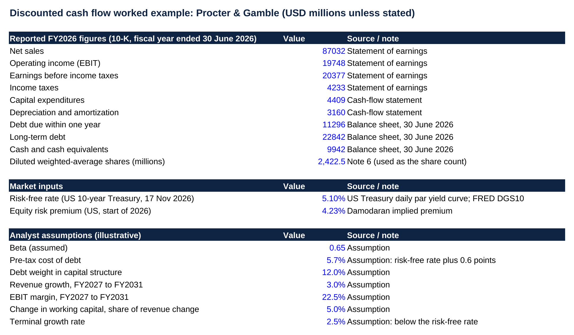
The example uses reported figures from the Procter & Gamble fiscal 2026 annual report on Form 10-K, for the year ended 30 June 2026. All amounts are in USD millions, and every forecast driver is an illustrative assumption, not a prediction.
Step 1: Anchor the forecast in reported results
Start from three years of reported history so that each assumption can be compared with what the business actually did.
| Item | 2024 | 2025 | 2026 |
|---|---|---|---|
| Net sales | 84,039 | 84,284 | 87,032 |
| Operating income | 18,545 | 20,451 | 19,748 |
| Operating cash flow | 19,846 | 17,817 | 19,556 |
| Capital expenditures | 3,322 | 3,773 | 4,409 |
| Depreciation and amortization | 2,896 | 2,847 | 3,160 |
| Operating cash flow less capital expenditures | 16,524 | 14,044 | 15,147 |
Step 2: Forecast unlevered free cash flow
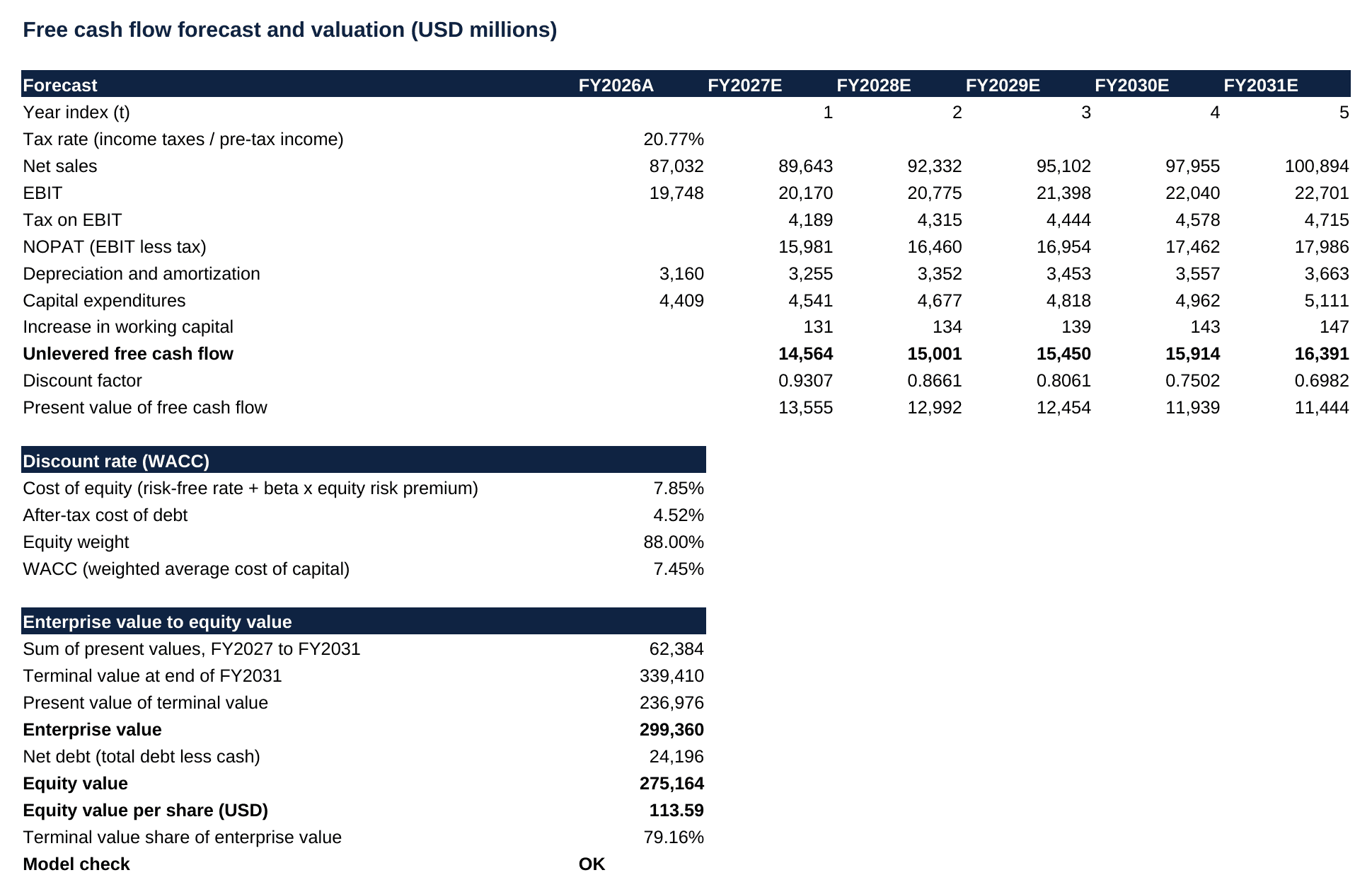
Unlevered free cash flow is the cash generated by operations before any payment to lenders. The Calculation sheet grows net sales 3.0% a year for five years and applies a 22.5% operating margin. Earnings before interest and taxes (EBIT) is taxed at the 20.77% effective rate implied by 4,233 of income taxes on 20,377 of pre-tax income, giving net operating profit after tax (NOPAT). Depreciation and amortization (3,160 in fiscal 2026) and capital expenditures are held at their fiscal 2026 shares of sales, 3.63% and 5.07% respectively, as an illustrative assumption. Depreciation and amortization is added back, capital expenditures are deducted, and working capital, the cash tied up in inventory and receivables net of payables, is assumed to absorb 5% of each year’s sales increase.
Every line is rounded to a whole number and each column adds exactly, so the first forecast year yields 14,564 of free cash flow, rising to 16,391 in year five. That path sits close to the 14,044 to 16,524 range of operating cash flow less capital expenditures reported over 2024 to 2026. This benchmark is levered, because operating cash flow is after interest, so it is only an approximate sanity check.
| Line | 2027 | 2028 | 2029 | 2030 | 2031 |
|---|---|---|---|---|---|
| Net sales | 89,643 | 92,332 | 95,102 | 97,955 | 100,894 |
| EBIT at 22.5% of sales | 20,170 | 20,775 | 21,398 | 22,040 | 22,701 |
| Tax on EBIT at 20.77% | 4,189 | 4,315 | 4,444 | 4,578 | 4,715 |
| NOPAT (EBIT less tax) | 15,981 | 16,460 | 16,954 | 17,462 | 17,986 |
| Depreciation and amortization at 3.63% of sales | 3,255 | 3,352 | 3,453 | 3,557 | 3,663 |
| Capital expenditures at 5.07% of sales | 4,541 | 4,677 | 4,818 | 4,962 | 5,111 |
| Increase in working capital | 131 | 134 | 139 | 143 | 147 |
| Unlevered free cash flow | 14,564 | 15,001 | 15,450 | 15,914 | 16,391 |
| Discount factor at 7.45% | 0.9307 | 0.8661 | 0.8061 | 0.7502 | 0.6982 |
| Present value of free cash flow | 13,555 | 12,992 | 12,454 | 11,939 | 11,444 |
Step 3: Build the discount rate
Free cash flow to the whole business is discounted at the weighted average cost of capital (WACC), the blended after-tax cost of equity and debt, as the Chartered Financial Analyst (CFA) Institute free cash flow valuation reading states for firm-level cash flows. The cost of equity is the return shareholders require, built from the risk-free rate (the yield on a government bond), beta (how strongly the stock moves with the overall market) and the equity risk premium (the extra return investors demand for holding stocks instead of bonds).
The inputs are a 5.10% US 10-year Treasury yield on 17 November 2026 and a 4.23% US equity risk premium at the start of 2026 from Damodaran. The premium dates from January 2026 and the yield from November 2026, a simplifying pairing.
With an assumed beta of 0.65, the cost of equity is 5.10% + 0.65 × 4.23% = 7.85%, rounded from 7.8495%. An assumed 5.7% pre-tax cost of debt, which is the interest rate on borrowing, becomes 5.7% × (1 − 20.77%) = 4.52% after tax. Weighting equity 88% and debt 12%, an assumed capital structure, gives a WACC of 0.88 × 7.85% + 0.12 × 4.52% = 7.45%.
Step 4: Add terminal value and bridge to equity value
Terminal value at the end of year five equals the final year’s free cash flow, grown once at 2.5% and divided by the gap between the WACC and that growth rate: 16,391 × 1.025 ÷ (7.45% − 2.5%) = 339,410. Discounted back five years at a factor of 0.6982, it is worth 339,410 × 0.6982 = 236,976 after rounding. Adding the 62,384 present value of the five forecast years gives an enterprise value of 299,360.
Subtracting net debt of 24,196 (debt of 34,138 less cash of 9,942) leaves an equity value of 275,164. Divided by 2,422.5 million diluted weighted-average shares, used as a simplifying proxy for period-end shares, that is 113.59 USD per share. Leases, pension deficits and noncontrolling interests are outside this simplified bridge, and a full valuation should deduct them. Terminal value is 79.2% of enterprise value.
The workbook cells behind these steps use plain formulas, rounded as in the tables.
| Line | Cell | Formula |
|---|---|---|
| Free cash flow, year 1 | Calculation!D13 | =D9+D10-D11-D12 |
| Discount factor, year 1 | Calculation!D14 | =1/(1+$C$21)^D4 |
| WACC | Calculation!C21 | =C20*C18+Inputs!C22*C19 |
| Terminal value | Calculation!C25 | =H13*(1+Inputs!C26)/(C21-Inputs!C26) |
| Enterprise value | Calculation!C27 | =C24+C26 |
Step 5: Stress the result with sensitivity analysis
A sensitivity analysis is a table that shows how the output changes when key inputs move. The Results sheet recomputes value per share for five WACC levels and five terminal growth rates using live formulas. Lowering WACC by half a point lifts value per share to 127.50, up 12.2%, while raising it by half a point cuts it to 102.23, down 10.0%. Raising terminal growth from 2.5% to 3.0% adds 10.1%, reaching 125.11.
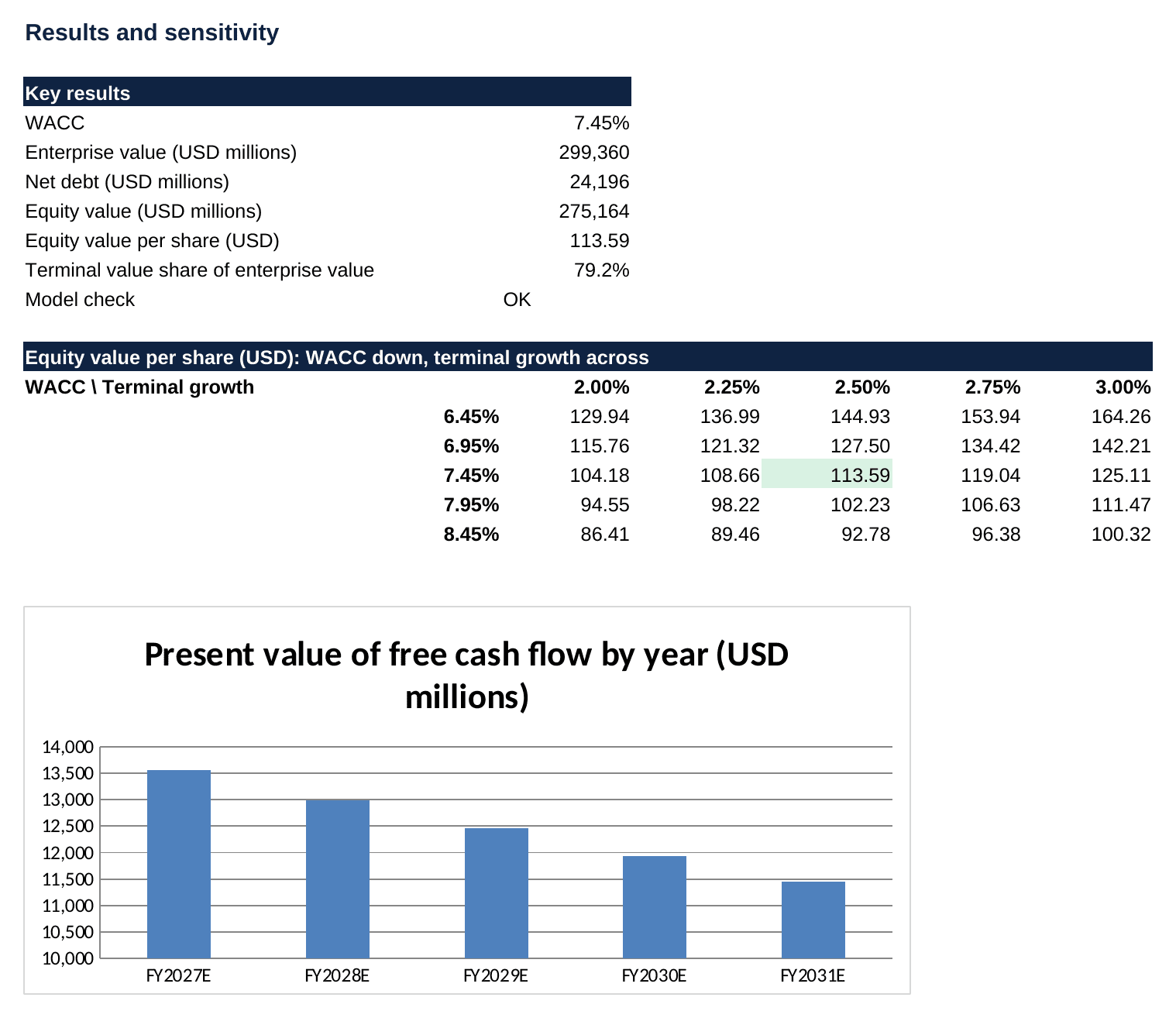
A check cell on the Calculation sheet reads OK only when enterprise value reconciles two ways, WACC exceeds terminal growth, and equity value equals enterprise value less net debt.
Common DCF Mistakes and the Check for Each
The discount rate and the terminal value are where input errors have the largest effect, because small changes compound there. The sensitivity grid above shows the effect in numbers. Two anchors: the 5.10% US 10-year Treasury yield on 17 November 2026 and a 4.23% US equity risk premium at the start of 2026 show the rates a model should stay consistent with, and the example’s terminal growth sits below that yield.
| Mistake | Why it distorts value | Check |
|---|---|---|
| Terminal growth above economic growth | Damodaran writes that the constant growth rate cannot be greater than the overall growth rate of the economy | Compare growth with long-run economic growth and the Treasury yield |
| Discounting firm-level cash flow at cost of equity | Overstates the rate and understates value | Use WACC for unlevered cash flow |
| Valuing a peak or trough year forever | One abnormal year gets capitalized into the terminal value | Average margins across a cycle |
| Capital expenditures below depreciation in perpetuity | A growing business cannot shrink its asset base | Keep terminal reinvestment above depreciation |
| Forgetting net debt | Enterprise value is not shareholder value | Subtract debt, add cash |
Frequently Asked Questions
How many years should a DCF forecast cover?
Five to ten years is typical, long enough for growth and margins to settle before the terminal value takes over. A mature, stable company can use five explicit years, as in this example, while a fast-growing business may need ten so growth fades gradually instead of dropping to the perpetual rate at once. The test is whether the final forecast year could repeat indefinitely.
Should the discount rate change from year to year?
Most models hold one rate across all years, which is the simplest approach and usually adequate. A changing rate becomes useful when the capital structure is expected to shift materially, for instance during a leveraged acquisition that is repaid over time. In that case the model needs a separate rate for each period, and discount factors are built by multiplying the yearly factors together.
Is a higher equity value per share the same as a buy signal?
No. The 113.59 figure is an output of stated assumptions and was never compared with a market price, because a DCF answers what the cash flows are worth under those inputs. Investors then compare that estimate with the traded price and with ranges from other methods. If a plausible change in WACC or growth flips the conclusion, the model is signalling uncertainty, not a clear opportunity.
Why discount at year end instead of mid-year?
Year-end discounting treats each year’s cash flow as arriving on the final day, which is easy to follow and slightly conservative. Mid-year discounting assumes cash arrives evenly through the year and shifts every exponent down by half a year, raising the present value of the forecast cash flows by about 3.7% at a 7.45% WACC. Either convention is acceptable if applied consistently and disclosed with the other assumptions.
Which cells in a DCF workbook should be hard-coded?
Only inputs should be typed in: reported figures, market data and labelled assumptions. Every other cell should be a formula, including the sensitivity grid, so changing one input updates the whole model. A single check cell that confirms the valuation reconciles catches broken links early. Pasted values over formulas quietly break the link between inputs and results, so no reviewer can trust the output.
Conclusion
A DCF model is only as reliable as its discount rate, its terminal assumptions and the discipline of its inputs, and the Procter & Gamble example shows that terminal value alone can carry 79.2% of enterprise value. Practitioners who want a ready structure can start from the eFinancialModels Free Discounted Cash Flow (DCF) Valuation Model Template.