0 ITEMS

Remove the Green Triangle in Excel: 3 Methods
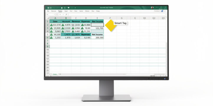
Excel’s green triangle is a built-in error indicator that flags potential data problems — and knowing when to remove it versus when to heed it can save you from costly spreadsheet mistakes.
Key Takeaways
- Excel displays green triangles in the upper-left corner of a cell when its background error-checking engine detects 1 of 8 specific rule violations.
- Method 1 (global disable) takes 5 clicks through File > Options > Formulas and removes all green triangles across every worksheet permanently.
- Method 2 (cell-by-cell Ignore Error) suppresses the triangle for a specific cell without changing any global setting — the right choice for shared workbooks.
- Method 3 (fix the root cause) uses Convert to Number, formula consistency corrections, or IFERROR wrapping to eliminate the underlying issue entirely.
- A VBA macro can batch-clear error indicators across all sheets in a workbook in under 2 seconds, saving hours of manual clicking on large files.
- Disabling background error checking on worksheets with 10,000+ rows can measurably reduce recalculation overhead, because Excel no longer evaluates each cell against 8 rule conditions on every change.
- Never disable error checking in financial models under audit, regulatory filings, or collaborative workbooks where a missed formula inconsistency could propagate silently.
Understanding Excel’s Green Triangle Error System
The green triangle (also called an error indicator) is a small marker Excel places in the upper-left corner of a cell when its background error-checking engine detects a potential problem. It is not an error itself — it is a warning that something about the cell’s content differs from what Excel expects based on surrounding data or formula patterns.
When you click a cell carrying a green triangle, a small yellow diamond icon (the Smart Tag) appears to the left. Clicking that diamond opens a dropdown menu with options including the error type description, a suggested fix, help documentation, and the option to Ignore Error.
Excel’s error-checking rules are defined under File > Options > Formulas > Error Checking Rules. As Microsoft’s documentation on detecting errors in formulas explains, background error checking runs continuously while you work and evaluates each cell against all enabled rules.
You can enable or disable each of the 8 rules independently, which gives you surgical control over which warnings appear. That granularity matters in complex models, because Excel’s published specifications and limits allow a single formula to nest up to 64 levels of functions — ample room for the deliberate formula variations that trigger false warnings.
This means complex formula chains can trigger multiple error rules simultaneously — another reason understanding each rule independently is valuable.
The Error Checking Rules section in Excel Options lets you enable or disable each of the 8 rule types independently.
The 8 Error Types That Trigger Green Triangles
Each green triangle maps to one specific rule. Understanding which rule fired tells you whether to fix the data or safely suppress the warning.
| Error Rule | What It Detects | Safe to Ignore? |
|---|---|---|
| Number stored as text | Numeric value entered or imported as text | Only if intentional |
| Inconsistent formula | Formula differs from adjacent range formulas | Rarely — check first |
| Formula omits cells | Formula skips cells adjacent to its range | Rarely — check first |
| Formula refers to empty cell | A cell reference in the formula is blank | Often yes |
| Unlocked cell with formula | Formula cell not locked for sheet protection | Depends on workflow |
| Two-digit year text date | Date text like “1/1/25” is ambiguous | Yes, if format is intentional |
| Data validation error | Cell value violates a validation rule | No — fix the data |
| Inconsistent calculated column | Table column formula breaks the pattern | Check before ignoring |
The most common trigger in financial work is “Number stored as text.” This happens frequently when data is pasted from external systems, PDFs, or web exports. Excel cannot sum or average text-formatted numbers, so a SUM formula silently returns a lower total than expected — a real financial risk. The scale of that risk grows with the dataset: Microsoft puts the worksheet ceiling at 1,048,576 rows, so a single bad paste can bury thousands of text-formatted values inside an otherwise clean model.
This means a single import operation can introduce hundreds of thousands of text-formatted number cells that each trigger this warning.
Method 1: Permanently Disable Error Checking Globally
The global disable method removes all green triangles from every cell in every worksheet by turning off background error checking entirely. Use this only when you are the sole owner of the workbook and you have independently verified data integrity.
Step-by-step (Excel 2016, 2019, 2021, and Microsoft 365 — same path for all versions):
- Click File in the top-left ribbon.
- Click Options at the bottom of the left panel. The Excel Options dialog opens.
- Click Formulas in the left sidebar.
- Under the Error Checking section, uncheck Enable background error checking.
- Click OK.
All green triangles disappear immediately. No restart required. To re-enable, follow the same path and recheck the box.
Selective rule disabling (recommended over full disable): If you only want to suppress one type of warning — for example, “Number stored as text” on a worksheet where text-format numbers are intentional — leave background error checking enabled and uncheck only that specific rule under Error Checking Rules in the same dialog. This preserves all other warnings.

Disabling background error checking globally takes 5 clicks and applies immediately to all worksheets — no restart required.
Method 2: Remove Green Triangles Cell-by-Cell Using Ignore Error
The Ignore Error method suppresses the green triangle for a specific cell without changing any global setting. This is the correct approach for shared workbooks, because it leaves error checking active for all other cells.
Steps:
- Click the cell showing the green triangle.
- A yellow diamond Smart Tag appears to the left of the cell. Click it.
- Read the error description at the top of the dropdown — confirm you understand why the triangle appeared.
- Click Ignore Error.
The triangle disappears for that cell. If you edit the cell later, Excel may re-evaluate it and the triangle could return.
To ignore errors across a range at once: Select the entire range first (e.g., A2:A500), then click the Smart Tag that appears and choose Ignore Error. Excel applies the suppression to all selected cells in one action.
To reset ignored errors (restore triangles you previously suppressed): Go to File > Options > Formulas > Error Checking and click Reset Ignored Errors.

The Smart Tag dropdown shows the specific error type and lets you Ignore Error for that cell without changing any global setting.
Method 3: Fix the Underlying Error Instead of Hiding the Indicator
Hiding the triangle is not the same as fixing the problem. For financial models, fixing the root cause is always the right approach.
Converting Numbers Stored as Text
This is the most impactful fix in finance work. Here’s the exact process:
- Select the column of text-formatted numbers (e.g., B2:B500).
- Click the Smart Tag on any cell in the selection.
- Choose Convert to Number.
Excel converts all selected cells from text to numeric format in one step. Your SUM and AVERAGE formulas now include every value.
Worked example: Suppose column B contains 500 revenue figures imported from an accounting system. All 500 are stored as text. Your SUM formula in B501 returns $0 because Excel cannot add text strings.
Here’s the math: Before conversion, =SUM(B2:B501) = $0. After selecting B2:B500 and clicking Convert to Number, =SUM(B2:B501) = $4,872,300. The difference is not a rounding error — it is the entire dataset being excluded from the calculation.
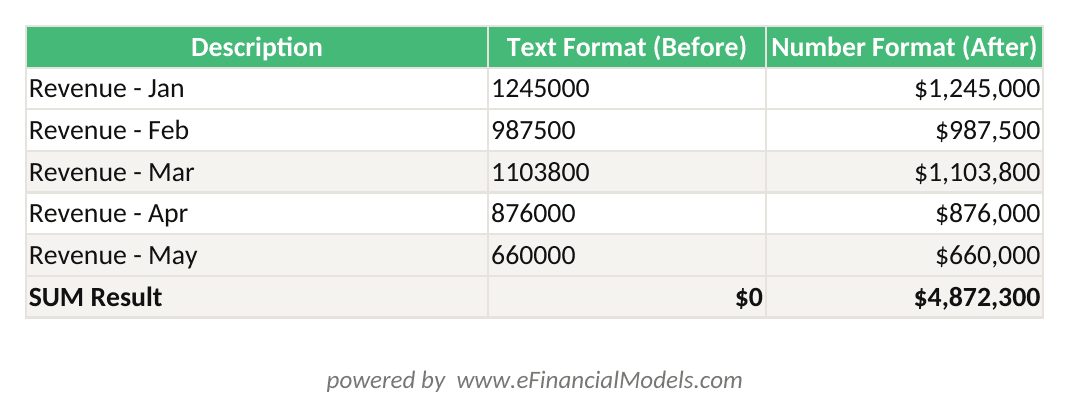
Before Convert to Number: SUM = $0. After conversion: SUM = $4,872,300. The formula is identical — only the cell format changes.
Fixing Inconsistent Formulas
Wrapping Formulas with IFERROR
IFERROR (a function that returns a custom value when a formula produces an error, instead of displaying #N/A, #VALUE!, or similar error codes) suppresses error display without hiding the underlying logic:
“`
=IFERROR(VLOOKUP(A2, RateTable, 2, 0), 0)
“`
This returns 0 when the VLOOKUP finds no match, instead of #N/A. Note: IFERROR hides the error from the user — use it only when a missing match is an expected, handled condition, not a data problem.
Numbers stored as text cause SUM to return $0 — Convert to Number fixes the root cause and the green triangle disappears automatically.*
Advanced Solution: VBA Macro for Batch Triangle Removal
For workbooks with dozens of sheets or thousands of flagged cells, a VBA macro (a recorded or written set of instructions that Excel executes automatically, stored in the workbook) clears all error indicators in seconds.
Paste this macro into the VBA Editor (Alt + F11 > Insert > Module):
“vba“
Sub ClearAllErrorIndicators()
Dim ws As Worksheet
Dim cell As Range
For Each ws In ThisWorkbook.Worksheets
For Each cell In ws.UsedRange
If cell.Errors.Item(xlEvaluateToError).Value = False Then
Dim i As Integer
For i = 1 To 9
cell.Errors.Item(i).Ignore = True
Next i
End If
Next cell
Next ws
MsgBox "Error indicators cleared across all sheets."
End Sub
Run the macro with F5 or by clicking Run. It loops through every worksheet and every used cell, setting the Ignore property to True for all 9 error indicator types. This is equivalent to manually clicking Ignore Error on every flagged cell — across every sheet in the file, and Excel allows a new workbook to be created with as many as 255 sheets.
This illustrates exactly why a VBA batch approach is far more practical than manually clicking Ignore Error sheet by sheet.
Important: This macro suppresses indicators — it does not fix underlying data issues. Run it only after you have reviewed and accepted the data quality in the workbook.
The VBA macro loops through every worksheet and cell in the workbook, setting Ignore to True for all 9 error indicator types in one run.
When You Should Keep Error Checking Enabled
Turning off error checking is not always the right call. There are 3 scenarios where keeping it enabled protects you.
1. Financial models under audit or review. External auditors and internal reviewers use green triangles as a quick scan for formula inconsistencies. A model where all triangles have been suppressed without fixing the underlying issues can mask real errors. Audit research collected by the European Spreadsheet Risks Interest Group (EuSpRIG) found that over 88% of spreadsheets examined contained errors, with formula inconsistencies among the most common categories.
Keeping error checking active gives auditors and model reviewers a reliable first-pass signal.
2. Collaborative workbooks. When multiple people edit the same file, a formula inconsistency introduced by one contributor may not be obvious to others. Error checking acts as a passive reviewer that flags deviations from established patterns.
3. Regulatory compliance filings. Any spreadsheet submitted to a regulator (tax authority, financial regulator, grant body) should have all formula warnings reviewed and resolved, not suppressed. Suppressing a warning without fixing the issue creates a documentation gap.

In audited financial models, green triangles serve as a first-pass signal for reviewers — suppressing them without fixing root causes creates documentation gaps.
Performance Considerations for Large Spreadsheets
Background error checking adds processing overhead on large datasets because Excel evaluates every cell against all enabled rules on each recalculation cycle. On worksheets with 10,000 or more rows, this overhead is measurable.
Microsoft’s guidance on error checking in Excel notes that background error checking runs continuously in the background, making it one of several features that contribute to recalculation time on large workbooks.
The practical impact depends on your hardware, but disabling error checking on a 50,000-row import sheet while keeping it enabled on your formula-heavy summary sheet is a reasonable performance optimization.
Comparison: Global Disable vs. Selective Rule Disable vs. Per-Cell Ignore
| Method | Scope | Reversible | Risk Level | Best For |
|---|---|---|---|---|
| Global disable | All cells, all sheets | Yes | High | Solo-owned, verified workbooks |
| Rule-level disable | All cells, specific rule | Yes | Medium | Known intentional patterns |
| Per-cell Ignore Error | Single cell or range | Yes | Low | Shared or audited workbooks |
| VBA batch ignore | All cells, all sheets | Partial | High | Large legacy files, one-time cleanup |
| Fix root cause | Single cell or range | N/A | None | All financial models |

Choosing the right removal method depends on whether the workbook is shared, audited, or performance-constrained.
Troubleshooting: Green Triangles That Won’t Disappear
Sometimes a green triangle persists even after you click Ignore Error. Here are the 3 most common causes and their fixes.
Problem 1: The cell is part of a protected sheet. Sheet protection (a feature that locks cells from editing) can prevent the Smart Tag from appearing or the Ignore Error action from saving. Unprotect the sheet (Review > Unprotect Sheet), apply Ignore Error, then re-protect.
Problem 2: The workbook is shared or co-authored in real time. In co-authoring mode via Microsoft 365, error indicator states may not sync immediately between users. Save and refresh the file, or have all co-authors close the file before applying global changes.
Problem 3: The error rule was re-enabled after you ignored it. If someone clicked Reset Ignored Errors in Excel Options, all previously ignored triangles return. Check with your team before resetting, and document which cells were intentionally suppressed.
Problem 4: The cell formula genuinely changed. Editing a cell resets its ignored-error state. If you update a formula, Excel re-evaluates it and may re-flag it. This is correct behavior — review the updated formula before suppressing the new warning.
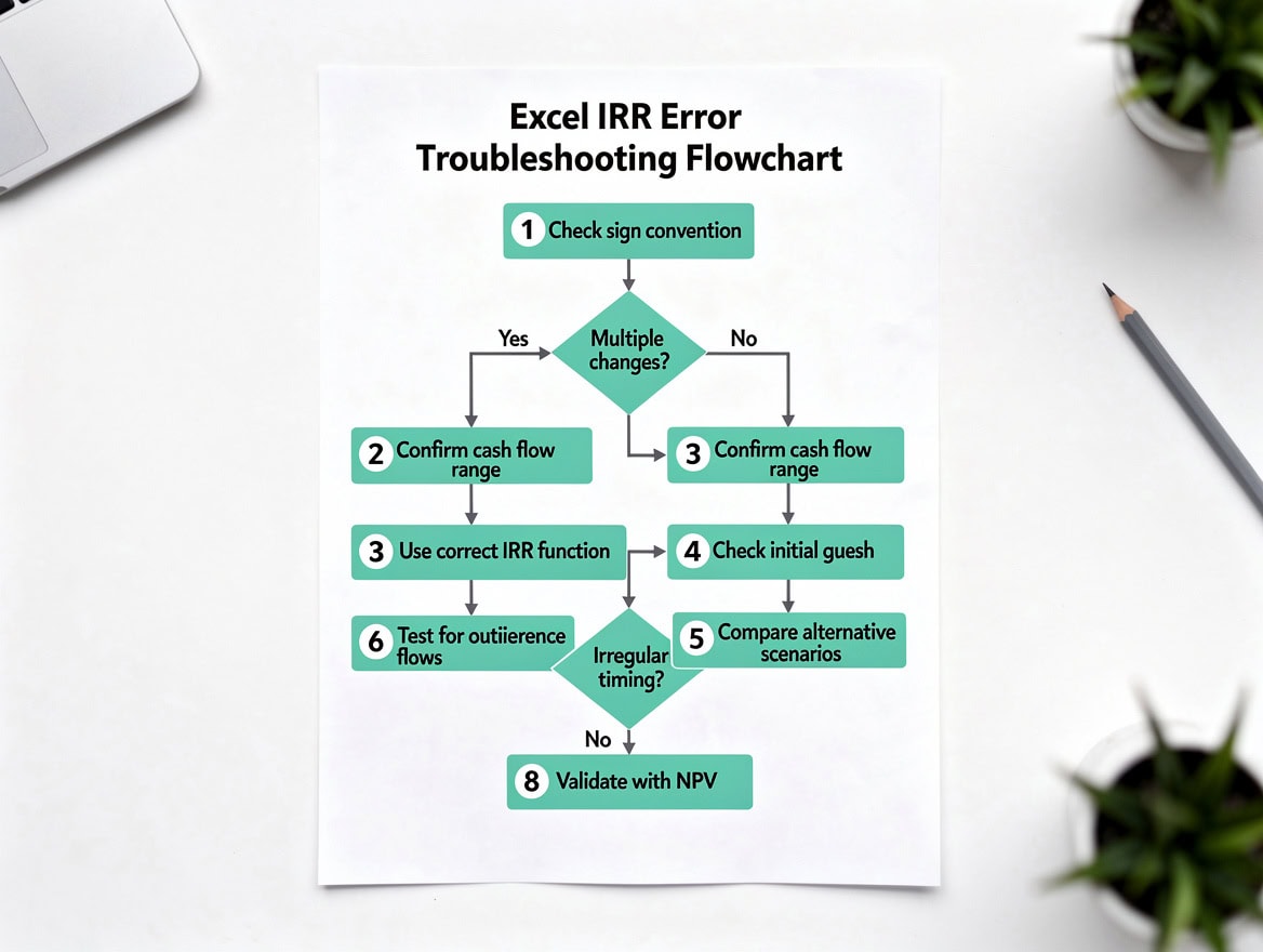
If a green triangle returns after you suppress it, one of these 4 conditions is almost always the cause.
Frequently Asked Questions
Why does Excel show a green triangle even when my formula is correct?
Excel’s error checking compares your formula against the pattern of surrounding cells, not against mathematical correctness. A formula can be perfectly correct and still trigger a green triangle if it differs from adjacent formulas. For example, if cells D2 through D49 all contain =BC and your cell D50 intentionally contains =B50C501.1 (a different rate), Excel flags D50 as inconsistent. The fix is to either click Ignore Error on D50 (confirming the difference is intentional) or add a comment to the cell documenting why it differs. This is one of the most common false-positive scenarios in financial modeling, where deliberate formula variations are standard practice.
What is the keyboard shortcut to navigate between green triangle cells?
There is no dedicated keyboard shortcut to jump between error-indicator cells the way F5 jumps to named ranges. However, you can use the Error Checking dialog: go to Formulas > Error Checking (in the Formula Auditing group) and Excel opens a dialog that steps through each flagged cell one by one, showing the error type and offering fix options. Press the Next button to advance. This is faster than manually scanning a large worksheet. Alternatively, pressing Alt + M, then Alt + E opens the Error Checking dialog via keyboard navigation without using the mouse.
Does removing the green triangle delete any data or change my formula?
No. Clicking Ignore Error or disabling background error checking does not alter cell values, formulas, or formatting in any way. It only suppresses the visual indicator. Your formula continues to calculate exactly as written. The only exception is Method 3 (fixing the root cause): actions like Convert to Number or editing a formula do change cell content, but those are deliberate corrections you initiate, not side effects of removing the triangle. Always distinguish between hiding the indicator and changing the underlying data.
Can I standardize error checking settings across my entire team’s Excel installations?
Yes, but it requires IT involvement. Excel stores error checking preferences in the Windows Registry under HKEY_CURRENT_USER\Software\Microsoft\Office\version\Excel\Options. An IT administrator can deploy a Group Policy Object (GPO) or a registry script that sets these values consistently across all machines in a domain. For Microsoft 365 deployments managed through the Microsoft 365 Admin Center, the Office Cloud Policy service allows administrators to configure Excel options including error checking rules and push them to all licensed users. This ensures that a financial modeling team, for example, all see the same set of active error rules without each person manually configuring their own Excel Options.
How do I remove green triangles in Excel Online or the Mac version?
Excel for the web (Excel Online) does not display green triangle error indicators at all — background error checking is a desktop-only feature as of Microsoft 365’s current web implementation. On Excel for Mac, the path is identical to Windows: Excel menu > Preferences > Error Checking, where you can uncheck Enable background error checking or adjust individual rules. The 8 error rule categories are the same on Mac. One difference: the Smart Tag on Mac appears as a small circle icon rather than a yellow diamond, but the Ignore Error option functions identically. Mac users running Excel 2019 or later have full parity with Windows on error checking features.
Is it safe to use the VBA macro to clear all error indicators in a financial model?
The VBA macro is safe in the sense that it does not change any cell values or formulas — it only sets the Ignore property on each error indicator to True, which is the same as manually clicking Ignore Error on every cell. However, “safe” in a financial modeling context means something more: you should only run this macro after a thorough manual review of the workbook’s data and formulas. Running it on an unreviewed model suppresses warnings that might be pointing to real errors — a number stored as text that causes a SUM to undercount, or a formula inconsistency that means one row uses a different interest rate than all others. Use the macro as a final cleanup step, not a first step.
Why do green triangles reappear after I remove them?
Green triangles return when 3 things happen: the cell is edited (Excel re-evaluates it from scratch), someone clicks Reset Ignored Errors in Excel Options (which clears all suppression states across the workbook), or a new paste or import operation introduces fresh data that triggers a rule. In collaborative workbooks, a co-author editing a cell you previously suppressed will cause the triangle to reappear for them and potentially sync back to you. The most durable solution is always to fix the root cause rather than suppress the indicator, because a fixed cell does not re-trigger the rule even after editing.
Conclusion
Green triangles in Excel are not bugs — they are Excel’s error-detection system doing its job. The right response depends on context: fix the root cause in financial models, use per-cell Ignore Error in shared workbooks, and consider a global disable only for verified, solo-owned files where the overhead outweighs the benefit.
For finance and accounting teams who want workbooks pre-configured with professional error-checking standards, I recommend downloading the Excel financial model templates from EFM — each template is built with formula consistency and data integrity practices already in place, so you spend less time managing error indicators and more time on analysis.