Discount Cash Flows in Excel: Step-by-Step DCF Guide

Discounting cash flows in Excel turns a theoretical valuation concept into a working spreadsheet you can interrogate, stress-test, and present to stakeholders in under an hour.

Key Takeaways

• Terminal value typically accounts for 60–80% of total enterprise value in a standard 5-year DCF model, making your long-term growth assumption the single most consequential input.
• The perpetuity growth rate in a DCF should never exceed the long-run nominal GDP growth rate — for developed markets, that ceiling sits around 2–3% annually.
• WACC (Weighted Average Cost of Capital) ranges from roughly 6% for large-cap utilities to 15%+ for early-stage technology companies, depending on capital structure and beta.
• Excel’s XNPV function is more accurate than NPV for real-world DCF models because it accounts for exact cash flow dates rather than assuming equal annual intervals.
• A 1-percentage-point change in the discount rate can shift enterprise value by 10–20% in a typical 5-year projection, which is why sensitivity tables are non-negotiable.
• Circular references — where a formula refers back to its own cell — are the most common structural error in Excel DCF models and can silently corrupt every output.
• Color-coding inputs (blue font), calculations (black font), and hard-coded checks (green font) is the industry-standard convention used by Big 4 advisory teams.

What Is DCF and Why Excel Is the Right Tool

A Discounted Cash Flow (DCF) model estimates what a business is worth today by projecting the cash it will generate in the future and converting those future amounts into present-day dollars using a discount rate. Excel is the preferred tool because it handles iterative calculations, scenario switching, and data tables natively — no specialist software required.

The core logic rests on the time value of money: a dollar received three years from now is worth less than a dollar today because today’s dollar can be invested and earn a return. The discount rate captures both that opportunity cost and the risk that the projected cash flows may not materialize.

Research consistently shows that forecast accuracy degrades sharply beyond a 5-year horizon. According to a study published in the Journal of Financial Economics, analyst earnings forecasts lose statistical reliability after approximately 2–3 years, which is why most professional DCF models cap explicit projections at 5–10 years and rely on a terminal value for everything beyond that window.

For a deeper look at how NPV and DCF connect, the EFM DCF model template library provides ready-built structures you can adapt immediately.

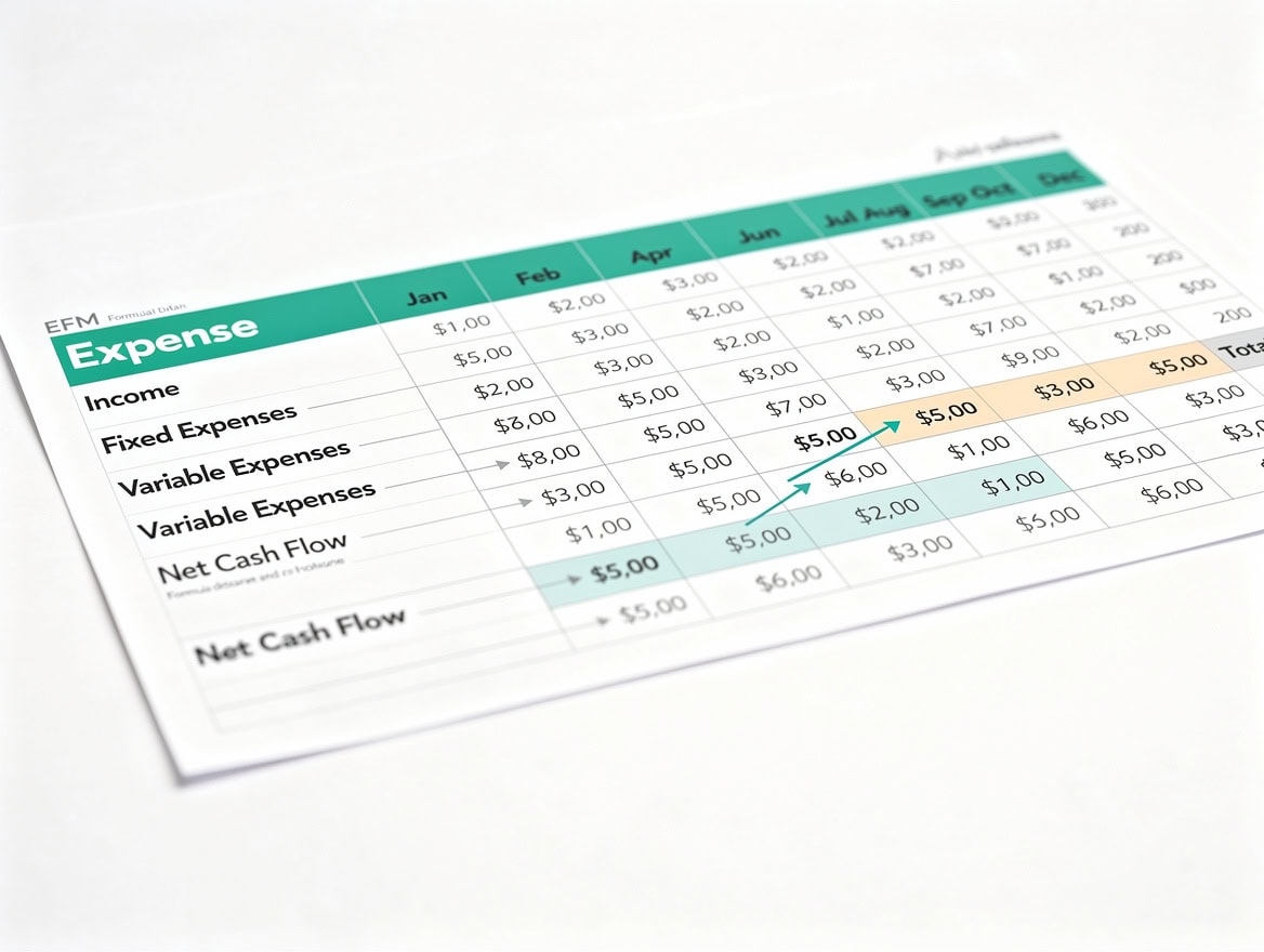
Each future cash flow shrinks in present-value terms as the discount period lengthens — the mathematical foundation of every DCF model.

Setting Up Your Excel DCF Worksheet Structure

A clean worksheet structure prevents errors and makes peer review faster. Organize your DCF across four dedicated tabs: Assumptions, Projections, Valuation, and Sensitivity.

Assumptions tab: Every input lives here — risk-free rate, beta, market risk premium, tax rate, revenue growth rates, capex as a percentage of revenue, and working capital days. Color all input cells with blue font. Never bury an assumption inside a formula.

Projections tab: This tab pulls from Assumptions and builds the income statement bridge to free cash flow. All cells here contain formulas, never hard-coded numbers. Use black font for calculated cells.

Valuation tab: Discounts the projected free cash flows, adds terminal value, and bridges from enterprise value to equity value.

Sensitivity tab: Houses two-variable data tables (explained in the sensitivity section below).

Lock all formula cells using Excel’s Review > Protect Sheet function after the model is complete. This prevents accidental overwrites during presentations. Excel’s Protect Sheet feature supports up to 16 individual permission options (Microsoft) that you can selectively enable or disable when restricting access to formula cells.

Separating inputs from calculations across dedicated tabs is the single most effective way to prevent formula errors in a DCF model.

Projecting Free Cash Flows in Excel: Formula Breakdown

Free Cash Flow to the Firm (FCFF) is the cash a business generates after covering operating expenses and capital investment, before any payments to debt or equity holders. It’s the correct cash flow metric for an unlevered DCF (the most common type).

Here’s the formula chain, row by row, assuming Year 1 data starts in column C and the label column is A:

<!-- wp:code -->
<pre class="wp-block-code"><code>Row 5:  Revenue                    = C4 * (1 + Assumptions!B3)    prior year × growth rate
Row 6:  EBIT                       = C5 * Assumptions!B5          revenue × EBIT margin
Row 7:  NOPAT (Net Operating       = C6 * (1 - Assumptions!B8)    EBIT × (1 - tax rate)
        Profit After Tax)
Row 8:  Depreciation &amp; Amort.      = C5 * Assumptions!B9          revenue × D&amp;A %
Row 9:  Capital Expenditures       = -C5 * Assumptions!B10        negative: cash outflow
Row 10: Change in Working Capital  = -(C5 - B5) * Assumptions!B11 incremental WC need
Row 11: Free Cash Flow             = C7 + C8 + C9 + C10</code></pre>
<!-- /wp:code -->

Working capital (current assets minus current liabilities, excluding cash and short-term debt) increases as revenue grows, consuming cash. A company growing revenue by $10M with a 15% net working capital ratio needs $1.5M more cash tied up in receivables and inventory — that $1.5M reduces free cash flow in that year.

Free Cash Flow to the Firm starts at NOPAT, not net income — a distinction that matters most for capital-intensive businesses with large depreciation or capex.

Calculating WACC in Excel: Inputs and Formula

WACC (Weighted Average Cost of Capital) is the blended required return across all capital providers — equity holders and debt holders — weighted by their share of total capital. It serves as the discount rate in an unlevered DCF.

The formula is:

WACC = (E/V) × Ke + (D/V) × Kd × (1 - Tax Rate)

Where:

• E/V = equity as a proportion of total capital (market value)
• D/V = debt as a proportion of total capital
• Ke = cost of equity (calculated via CAPM)
• Kd = pre-tax cost of debt (yield on outstanding debt)
• Tax Rate = marginal corporate tax rate (the interest tax shield reduces the effective cost of debt)

Cost of equity via CAPM:

Ke = Risk-Free Rate + Beta × Market Risk Premium

For 2024–2025 inputs: the 10-year US Treasury yield (the standard risk-free rate proxy) has ranged between 4.2% and 4.8%. According to Damodaran’s annual survey data published by NYU Stern, the implied equity risk premium for the US market was approximately 4.6% as of January 2025. Beta values vary by sector: utilities average around 0.5, consumer staples around 0.6, and technology companies often range from 1.2 to 1.8.

In Excel, with inputs on the Assumptions tab:

B14 (Cost of Equity) = B4 + B5 * B6         Risk-Free + Beta × ERP
B15 (After-tax Kd)   = B7 * (1 - B8)        Kd × (1 - Tax Rate)
B16 (WACC)           = B9*B14 + B10*B15     Equity weight×Ke + Debt weight×Kd(1-t)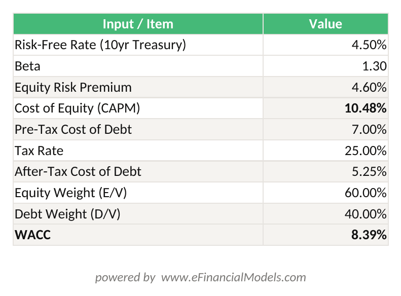

WACC = (60% × 12.3%) + (40% × 5.25% × 75%) = 9.8% — the discount rate applied to all projected free cash flows in the DCF model.

Discounting Cash Flows to Present Value: NPV in Practice

Once you have projected free cash flows and a WACC, discounting each year’s cash flow to present value is straightforward. Excel offers two functions: NPV and XNPV.

NPV(rate, value1, value2, ...) assumes cash flows arrive at equal annual intervals. XNPV(rate, values, dates) accepts actual dates, making it more accurate when cash flows don’t fall exactly 12 months apart. For most annual DCF models, NPV is sufficient, but XNPV is the professional standard. Excel’s XNPV function can handle a range of up to 254 value-date pairs (Microsoft), making it well-suited for multi-year DCF models with granular cash flow schedules.

Mid-year convention: Standard DCF assumes cash flows arrive at year-end. In reality, cash flows arrive throughout the year. The mid-year convention adjusts the discount exponent from n to n - 0.5, pulling present values slightly higher. To apply it in Excel:

PV of Year n CF = FCF_n / (1 + WACC)^(n - 0.5)

For a model without mid-year convention, the present value formula in cell C20 (Year 1 PV) is:

= C11 / (1 + Valuation!B3)^C2

Where C11 is the Year 1 FCF and C2 is the year number (1, 2, 3…).

Sum all discounted cash flows:

B25 (PV of FCFs) = SUM(C20:G20)     Years 1–5 present values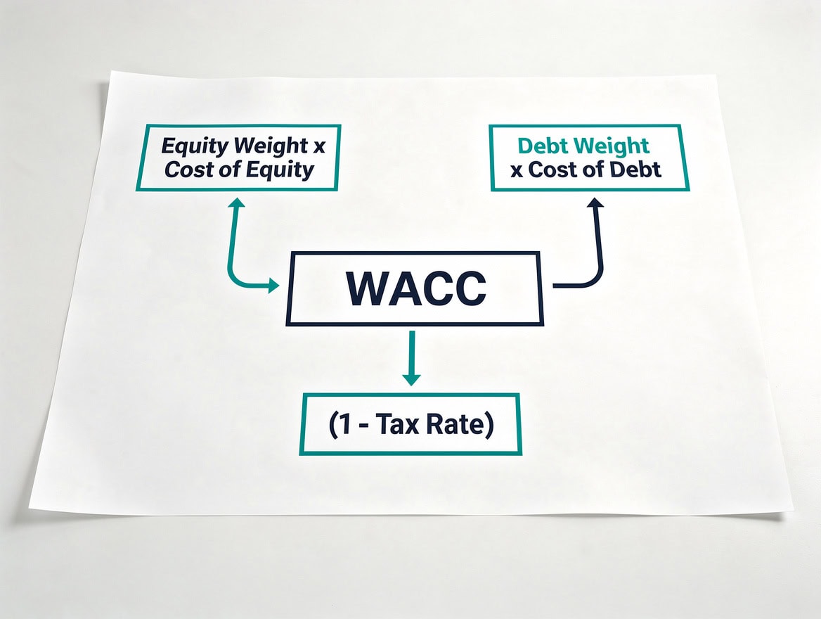

WACC blends two required returns: equity holders demand compensation for market risk (via beta), while debt holders receive an after-tax yield.

Terminal Value: Perpetuity Growth vs. Exit Multiple

Terminal value captures all cash flows beyond the explicit forecast period. Because it represents the bulk of enterprise value in most models — often 60–80% of the total — small changes in your assumptions create large swings in output.

Perpetuity Growth Model (Gordon Growth Model)

This method assumes the business grows at a constant rate forever after the forecast period:

Terminal Value = FCF_(n+1) / (WACC - g)

Where g is the perpetuity growth rate. In Excel:

B30 (Terminal Value) = G11 * (1 + Assumptions!B12) / (Valuation!B3 - Assumptions!B12)

The perpetuity growth rate g must stay below the long-run nominal GDP growth rate. For the US, the Congressional Budget Office projects long-run real GDP growth of approximately 1.8% annually; adding 2% inflation implies a nominal ceiling of roughly 3.8%. Using a g above this level implies the company will eventually be larger than the entire economy — an impossibility.

Exit Multiple Method

This method applies a market-derived EBITDA multiple to the final forecast year’s EBITDA:

Terminal Value = EBITDA_(Year n) × Exit Multiple

In Excel:

B31 (TV - Exit Multiple) = G_EBITDA * Assumptions!B13

Always calculate both methods and triangulate. A large gap between the two signals that either your growth rate or your multiple is out of line with market reality.

Discount the terminal value back to present value:

B32 (PV of Terminal Value) = B30 / (1 + Valuation!B3)^5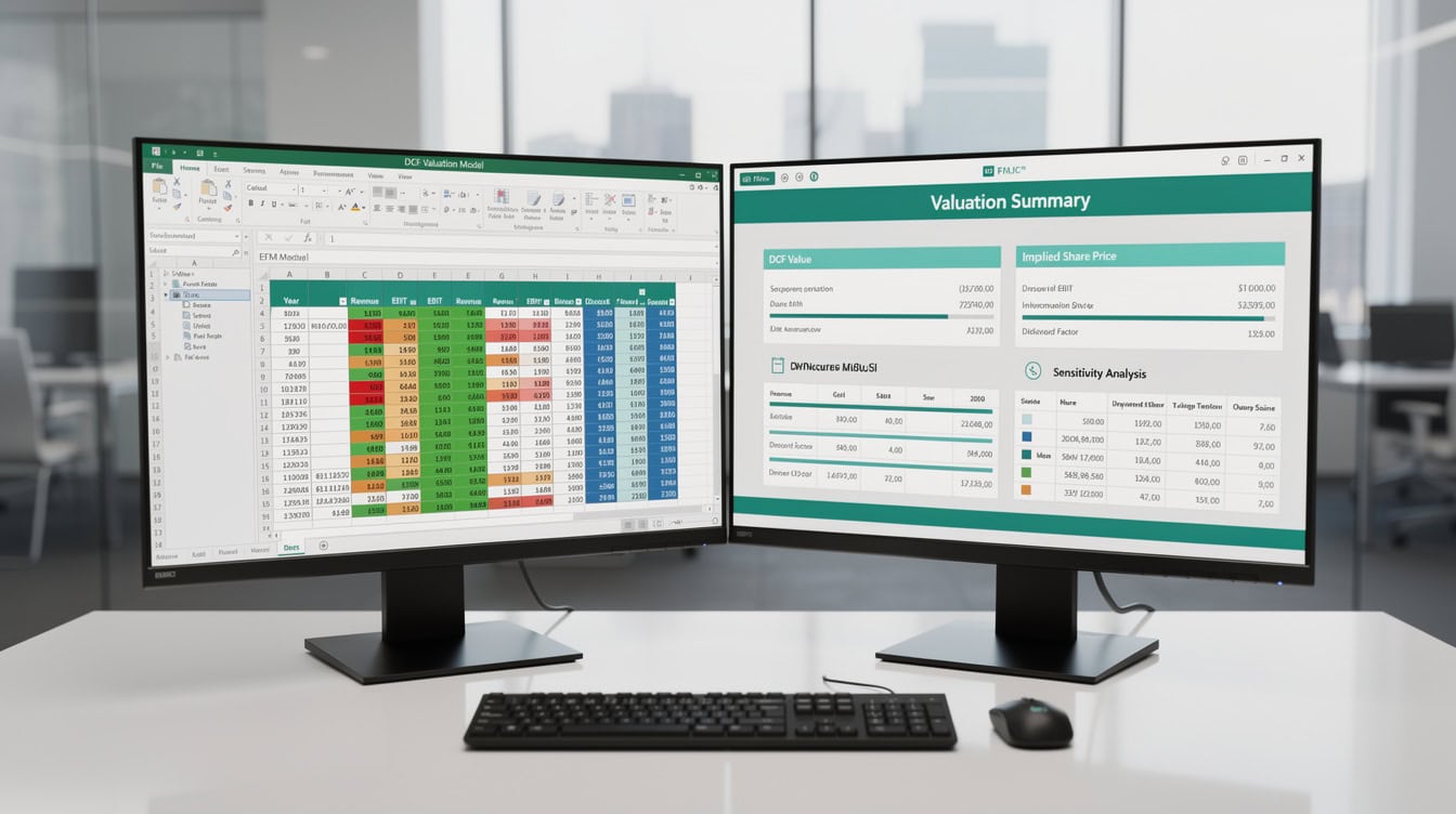

Running both terminal value methods and comparing results is a standard sanity check — a large gap signals that one assumption is out of line with market reality.

Worked Numerical Example: 5-Year DCF

Here’s the math for a simplified company with $50M in Year 1 revenue:

Inputs:

• Revenue growth: 10% per year
• EBIT margin: 20%
• Tax rate: 25%
• D&A: 3% of revenue
• Capex: 5% of revenue
• Change in working capital: 2% of revenue increment
• WACC: 10%
• Perpetuity growth rate: 2.5%

Year 1 FCF calculation:

• Revenue: $50.0M
• EBIT: $50.0M × 20% = $10.0M
• NOPAT: $10.0M × (1 – 25%) = $7.5M
• D&A: $50.0M × 3% = $1.5M
• Capex: -$50.0M × 5% = -$2.5M
• Change in WC: -(Year 1 Rev – Year 0 Rev) × 2% = -($50M – $45.5M) × 2% = -$0.09M (using implied prior year)
• FCF Year 1 = $7.5M + $1.5M – $2.5M – $0.09M = $6.41M

Present value of Year 1 FCF: $6.41M / (1.10)^1 = $5.83M

Repeating this for Years 2–5 and summing gives a PV of FCFs of approximately $24.1M.

Terminal value (perpetuity growth):

• Year 5 FCF (estimated): ~$9.8M
• TV = $9.8M × (1 + 2.5%) / (10% – 2.5%) = $10.05M / 7.5% = $133.9M
• PV of TV = $133.9M / (1.10)^5 = $83.2M

Enterprise Value = $24.1M + $83.2M = $107.3M

Note that the terminal value ($83.2M) represents 77.5% of total enterprise value — squarely within the typical 60–80% range. This is why your perpetuity growth rate assumption deserves more scrutiny than your Year 2 revenue forecast.

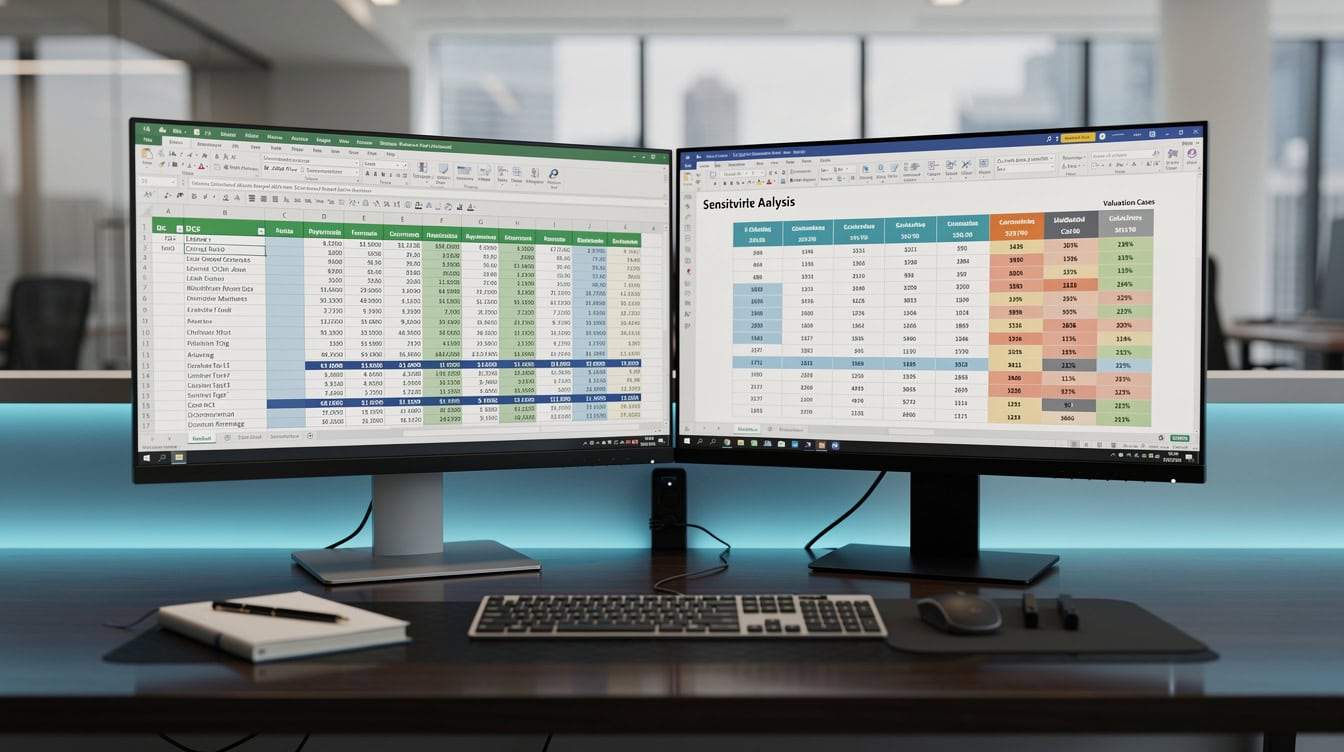
In this example, terminal value ($83.2M) represents 77.5% of the $107.3M enterprise value — consistent with the typical 60–80% range in professional DCF models.

Building Sensitivity Tables in Excel

Sensitivity analysis tests how enterprise value changes when you vary two key assumptions simultaneously. Excel’s Data Table feature (a two-variable data table) automates this without requiring you to manually change inputs. A single Excel workbook can contain up to 255 sheets (Microsoft), giving you ample room to dedicate separate tabs to assumptions, projections, valuation, and multiple sensitivity scenarios without hitting structural limits.

Setup steps:

1. Place your enterprise value formula in a reference cell (e.g., B40 = Valuation!B35).
2. In a new range, list WACC values across the top row (e.g., 8%, 9%, 10%, 11%, 12% in cells D42:H42).
3. List perpetuity growth rates down the left column (e.g., 1.5%, 2.0%, 2.5%, 3.0%, 3.5% in cells C43:C47).
4. In cell C42, enter a reference to your enterprise value formula: = B40.
5. Select the entire table range C42:H47, go to Data > What-If Analysis > Data Table, set Row Input Cell to the WACC cell and Column Input Cell to the growth rate cell, then click OK.

Excel populates every cell in the table automatically. The result is a grid showing enterprise value under 25 different combinations of WACC and growth rate.

Highlight the cell closest to your base-case assumptions in a different color so readers immediately see where the model’s central estimate sits.

A color-coded sensitivity table immediately shows which assumption combinations produce the widest valuation range — essential for investment committee presentations.

Common Excel DCF Errors and How to Fix Them

Even experienced analysts make structural mistakes that silently corrupt DCF outputs. Here are the 5 most common, with specific fixes.

1. Circular references in WACC: If your WACC formula references a debt schedule that itself references WACC (common in models with dynamic interest calculations), Excel will either error or iterate to a wrong answer. Fix: break the circularity by using prior-period debt balances in the interest calculation, or enable iterative calculation under File > Options > Formulas with a maximum of 100 iterations.
2. Hard-coded numbers inside formulas: Writing = 50000000 * 0.20 instead of = Revenue * EBIT_Margin makes the model impossible to audit and easy to break. Fix: every assumption must live in a named cell on the Assumptions tab. Reference it by cell address or named range.
3. Inconsistent time periods: Mixing annual and quarterly cash flows without adjusting the discount rate destroys accuracy. A 10% annual WACC applied to quarterly cash flows must be converted: (1 + 10%)^(1/4) - 1 = 2.41% per quarter. Fix: standardize all projections to the same period before discounting.
4. Forgetting to discount the terminal value: A common beginner error is adding the undiscounted terminal value to the sum of discounted cash flows. Fix: always divide terminal value by (1 + WACC)^n where n is the final projection year.
5. Using net income instead of free cash flow: Net income includes non-cash charges and ignores capex and working capital changes. Using it as a proxy for cash flow overstates value for capital-intensive businesses. Fix: always start from NOPAT and add back D&A, then subtract capex and working capital changes.

Each of these 5 errors can shift enterprise value by 20% or more — making a peer-review checklist as important as the model itself.

Interpreting DCF Output: Enterprise Value to Investment Decision

Once you have enterprise value (EV), bridge it to equity value and compare it to the current market price.

Equity Value = Enterprise Value – Net Debt + Cash

Net debt equals total interest-bearing debt minus cash and cash equivalents. If the company has $107.3M enterprise value, $20M in debt, and $5M in cash:

Equity Value = $107.3M - $20M + $5M = $92.3M

If the company has 10 million shares outstanding, the implied share price is $9.23. Compare this to the current market price:

• If market price is $7.50, the stock trades at a 19% discount to intrinsic value — potentially undervalued.
• If market price is $11.00, the stock trades at a 19% premium — potentially overvalued.

DCF is one input, not a verdict. Cross-validate against trading multiples (EV/EBITDA, P/E) and precedent transactions before drawing conclusions. For a structured approach to multi-method valuation, the EFM forecasting template collection provides comparable company analysis frameworks alongside DCF outputs.

The final step of any DCF is comparing implied share price to market price — but always cross-validate with trading multiples before drawing investment conclusions.

DCF Model Best Practices: Templates, Color Coding, and Audit Trails

A professional DCF model is readable by someone who didn’t build it. These conventions make that possible.

Color coding standard (Big 4 convention):

• Blue font: hard-coded inputs (only on the Assumptions tab)
• Black font: formulas and calculations
• Green font: links from other tabs or external sources
• Red font: error checks (cells that should equal zero if the model balances)

Documentation: Add a Model Log tab recording the date, author, version number, and a one-line description of every material change. This creates an audit trail for regulatory or client review.

Error checks: Build a dedicated row of checks. For example, confirm that the sum of equity value plus net debt equals enterprise value. If the check cell shows anything other than zero, the model has an inconsistency.

Template structure: The EFM Excel financial model templates follow these conventions and include pre-built sensitivity tables, WACC calculators, and error-check dashboards. Starting from a validated template cuts model-build time significantly and reduces the risk of structural errors.

For KPI tracking alongside your DCF, the EFM KPI template library integrates operational metrics directly into financial projections.

Frequently Asked Questions

How do I discount cash flows in Excel using the NPV function?

Excel’s NPV(rate, value1, value2, …) function discounts a series of future cash flows at a constant rate and returns their combined present value. The syntax assumes the first cash flow occurs one period from now. If you have a Year 0 outflow (an initial investment), add it outside the NPV function: = NPV(WACC, C11:G11) + B11, where B11 is the Year 0 cash flow (typically negative). For irregular dates, use XNPV(rate, values, dates) instead. Always verify that your rate matches your cash flow period: an annual WACC applied to annual cash flows, a quarterly rate to quarterly flows.

What discount rate should I use in a DCF model?

For an unlevered DCF (the most common type), use WACC as the discount rate. WACC blends the cost of equity (calculated via CAPM: risk-free rate + beta × equity risk premium) and the after-tax cost of debt, weighted by each source’s share of total capital. As of 2025, a US large-cap industrial company might have a WACC of 8–10%, while a high-growth technology company could see 12–15%. The risk-free rate input should use the 10-year US Treasury yield, which has ranged between 4.2% and 4.8% in 2024–2025 according to Federal Reserve H.15 data. Never use a single generic discount rate across all industries.

Why does terminal value dominate the DCF result?

Terminal value captures all cash flows beyond the explicit forecast period, which in a growing business represents the majority of total value. In a standard 5-year DCF, terminal value typically accounts for 60–80% of enterprise value. This concentration is mathematically inevitable: a business worth $100M today that grows at 2.5% forever generates most of that value in years 6 through infinity, not in years 1 through 5. The practical implication is that your perpetuity growth rate assumption matters far more than your Year 3 revenue forecast. Keep the growth rate below long-run nominal GDP growth (roughly 3–4% for developed markets) to avoid implying the company will eventually outgrow the entire economy.

What is the difference between NPV and DCF in Excel?

DCF (Discounted Cash Flow) is the overall valuation methodology: project future cash flows, discount them to present value, and sum the results. NPV (Net Present Value) is a specific Excel function that performs the discounting and summing step. In practice, analysts use the NPV or XNPV function as the mechanical tool inside a DCF model. The distinction matters because NPV in Excel does not automatically include terminal value — you must calculate terminal value separately, discount it, and add it to the NPV function’s output. A complete DCF model therefore looks like: Enterprise Value = NPV(WACC, FCF_Year1:FCF_Year5) + PV_of_Terminal_Value.

How do I build a sensitivity table for a DCF in Excel?

Use Excel’s two-variable Data Table under Data > What-If Analysis > Data Table. Place your enterprise value formula in a corner cell of the table. List one variable (e.g., WACC) across the top row and a second variable (e.g., perpetuity growth rate) down the left column. Select the entire table range, open the Data Table dialog, assign the row input cell to your WACC assumption cell and the column input cell to your growth rate assumption cell, then click OK. Excel calculates enterprise value for every combination automatically. A 5×5 table testing WACC from 8% to 12% and growth from 1.5% to 3.5% gives you 25 scenarios in seconds, revealing how sensitive your valuation is to each assumption.

What are the most common errors in Excel DCF models?

The 5 most damaging errors are: (1) circular references in the WACC or interest calculation that cause Excel to iterate incorrectly; (2) hard-coded numbers embedded in formulas rather than referenced from an Assumptions tab; (3) mixing time periods without adjusting the discount rate (annual WACC applied to quarterly cash flows); (4) forgetting to discount the terminal value back to the present — a surprisingly common mistake that inflates enterprise value by 60–80%; and (5) using net income as a proxy for free cash flow, which ignores capex and working capital changes. Each of these errors can shift enterprise value by 20% or more, which is why peer review and a dedicated error-check row are essential before sharing any model.

How do I convert enterprise value to equity value in Excel?

Equity value equals enterprise value minus net debt (total interest-bearing debt minus cash and cash equivalents). In Excel: Equity Value = Enterprise_Value – Total_Debt + Cash. If the company also has minority interests or preferred stock, subtract those as well: Equity Value = EV – Debt + Cash – Minority_Interest – Preferred_Stock`. Divide equity value by diluted shares outstanding (including options and convertible instruments on a treasury-stock basis) to arrive at intrinsic value per share. Compare that figure to the current market price to determine whether the stock appears undervalued or overvalued relative to your DCF assumptions.

Conclusion

Building a DCF model in Excel is a skill that compounds: each model you build makes the next one faster and more accurate. The mechanics are straightforward once you separate the four components — free cash flow projection, WACC calculation, present value discounting, and terminal value — and handle each in its own worksheet section. The real edge comes from disciplined assumptions, rigorous error checks, and sensitivity tables that show stakeholders the range of outcomes rather than a single point estimate.

I recommend downloading the EFM professional DCF valuation model as your starting framework. It includes a pre-built WACC calculator, mid-year convention toggle, both terminal value methods, a two-variable sensitivity table, and a full error-check dashboard — everything covered in this guide, already structured and ready to populate with your company’s data.

by Apollo Financial Models

Hospitality (Hotel) Financial Model and Valuation – 10-year Projections

Average rating:Submit Rating

Welcome to the Hospitality (Hotel) Company Financial Model and Valuation, your ultimate solution for making well-informed investment decisions in the ... read more

•  Free PDF – $0.00 Version 1
•  Excel Model – $24.99 Version 1

Add to wish list

Purchase Checkout Added to cart Excluding 0% tax

by Apollo Financial Models

Car Dealership Financial Model and Valuation – Financial Projections

Average rating:Submit Rating

Welcome to the Car Dealership Company Financial Model and Valuation, your ultimate solution for making well-informed investment decisions in the car d... read more

•  Free PDF – $0.00 Version 1
•  Excel Model – $24.99 Version 1

Add to wish list

Purchase Checkout Added to cart Excluding 0% tax

by Profit Vision

Fruit Processing Facility – 10 Year Financial Model

Average rating:Submit Rating

Financial Model providing a dynamic up to 10-year financial forecast for a startup Fruit Processing Facility.

•  Financial Model - Light Version – $99.00 Version 1
•  Financial Model - Premium Version – $129.00 Version 1
•  PDF Free Demo – $0.00 Version 1

Add to wish list

Purchase Checkout Added to cart Excluding 0% tax

by eFinancialModels

Solar Energy Financial Model

Average rating:

The Solar Energy Financial Model Spreadsheet Template in Excel assists you in preparing a sophisticated financial forecast for a utility-scale solar p... read more

•  PREMIUM – $149.95 Version 7.4
•  PRO – $129.95 Version 7.4
•  BASIC – $99.95 Version 7.4
•  PDF Demos – $0.00 Version 7.4

Add to wish list

Purchase Checkout Added to cart Excluding 0% tax

by Street Fox Advisors

Private Equity Fund Model (Investor Cashflows)

Average rating:

The Private Equity Fund Cashflows Model helps LPs and GPs analyze fund cash flows, returns, and distributions across investor, manager, and portfolio ... read more

•  PDF Demo version – $0.00 Version 3
•  European Waterfall – $105.00 Version 3
•  American Waterfall – $125.00 Version 3

Add to wish list

Purchase Checkout Added to cart Excluding 0% tax

by eFinancialModels

Financial Model for Mobile App | Mobile App Business Plan

Average rating:

The Mobile App Financial Plan Template in Excel allows you to develop financial projections when launching a new business centered around an app insta... read more

•  PREMIUM – $209.95 Version 7.3
•  PRO – $159.95 Version 7.3
•  BASIC – $109.95 Version 7.3
•  PDF Demo Versions – $0.00 Version 7.3

Add to wish list

Purchase Checkout Added to cart Excluding 0% tax

by eFinancialModels

Pharma Biotech Valuation Model Template (Risk-Adjusted)

Average rating:

The Pharma Biotech Valuation Model Template calculates the risk-adjusted DCF Value of a Pharma or Biotech Startup Company with several products under ... read more

•  Full Excel Model - PREMIUM – $199.95 Version 2.2
•  Full Excel Model - BASIC – $149.95 Version 2.2
•  PDF Demo Previews – $0.00 Version 2.2

Add to wish list

Purchase Checkout Added to cart Excluding 0% tax

by eFinancialModels

Expert Financial Modeling Services

Average rating:

Hire professional eFinancialModels financial modelers for customized financial modeling services tailored to support your financial decision-making.

•  1 Hour – $200.00 Version 1.0
•  2 Hours – $400.00 Version 1.0
•  3 Hours – $600.00 Version 1.0
•  4 Hours – $800.00 Version 1.0
•  5 Hours – $1,000.00 Version 1.0
•  6 Hours – $1,200.00 Version 1.0
•  8 Hours – $1,600.00 Version 1.0
•  1.5 Days – $2,400.00 Version 1.0
•  2 Days – $3,200.00 Version 1.0

Add to wish list

Purchase Checkout Added to cart Excluding 0% tax

by eFinancialModels

SaaS Business Financial Model

Average rating:

The SaaS Business financial model offers valuable assistance in preparing a budget and multi-year financial plan for a Software as a Service (SaaS) bu... read more

•  Premium Excel Model – $199.95 Version 8.2
•  Pro Excel Model – $149.95 Version 8.2
•  Basic Excel Model – $99.95 Version 8.2
•  PDF Demo – $0.00 Version 8.2

Add to wish list

Purchase Checkout Added to cart Excluding 0% tax

by eFinancialModels

Upstream Oil & Gas Project Analysis

Average rating:

The Upstream Oil & Gas Project Financial Model Template in Excel empowers you to project and dissect your impending Oil and Gas drilling ventures. Pre... read more

•  Pro - Full Excel Model – $159.95 Version 8.3
•  Basic - Full Excel Model – $119.95 Version 8.3
•  PDF Demo Versions – $0.00 Version 8.3

Add to wish list

Purchase Checkout Added to cart Excluding 0% tax

by eFinancialModels

Manufacturing Startup Feasibility Model

Average rating:

Launching a manufacturing startup can be complex, and securing financing requires a solid financial plan. Our Manufacturing Startup Financial Feasibil... read more

•  PREMIUM Excel Version – $129.95 Version 2.41
•  BASIC Excel Version – $89.95 Version 2.41
•  PDF DEMO Versions – $0.00 Version 2.41

Add to wish list

Purchase Checkout Added to cart Excluding 0% tax

by Profit Vision

Professional Financial Modeling Services – Profit Vision

Average rating:

Professional Financial Modeling - Tailor Made Services and assistance for your business needs.

•  Hourly Rate – $100.00 Version 1
   x 
•  Daily Rate – $800.00 Version 1
   x 

Add to wish list

Purchase Checkout Added to cart Excluding 0% tax

by Projectify

Projectify Custom Financial Modeling Services

Average rating:

Providing you professional custom Financial Modeling services and assistance for your business needs.

•  1 Hour – $115.00 Version 1
   x 
•  4 Hours – $460.00 Version 1
   x 
•  8 Hours – $800.00 Version 1
   x 
•  10 Hours – $900.00 Version 1
   x 
•  1.5 Days – $1,080.00 Version 1
   x 
•  2 Days – $1,440.00 Version 1
   x 

Add to wish list

Purchase Checkout Added to cart Excluding 0% tax

by eFinancialModels

Commercial Real Estate Valuation Model Template

Average rating:

A commercial real estate valuation model template assists in running a professional DCF Valuation for a commercial property such as an office building... read more

•  PDF Demo Versions – $0.00 Version 1
•  BASIC Excel Model Template – $59.00 Version 1
•  PRO Excel Model Template – $99.00 Version 1
•  PREMIUM Excel MODEL + Report Template – $199.00 Version 1

Add to wish list

Purchase Checkout Added to cart Excluding 0% tax

by smarthelping

All My Financial Models, Spreadsheets, Templates, and Tools: 120+

Average rating:

Lifetime access to all future templates as well! Here is a set of spreadsheets that have some of the most valuable logic in the world. I have been thr... read more

•  All My Excel Tools – $499.00 Version 1

Add to wish list

Purchase Checkout Added to cart Excluding 0% tax

by eFinancialModels

Real Estate Portfolio Financial Model

Average rating:Submit Rating

The Real Estate Portfolio Financial Model Template forecasts the financial performance when building a real estate portfolio. The model allows simulat... read more

•  Full Excel Version – $199.95 Version 2.7
•  PDF Demo Version – $0.00 Version 2.7

Add to wish list

Purchase Checkout Added to cart Excluding 0% tax

by eFinancialModels

Beverage Manufacturing Start-Up Financial Model

Average rating:

The beverage manufacturing industry is a dynamic and rapidly growing sector that caters to a diverse market ranging from soft drinks and juices to alc... read more

•  Excel Model – $249.95 Version 5.3
•  PDF Demo – $0.00 Version 5.3

Add to wish list

Purchase Checkout Added to cart Excluding 0% tax

by eFinancialModels

Solar + BESS Financial Model Template (Excel, 40-Year Forecast)

Average rating:

A Solar + BESS template is a pre-built Excel financial model that forecasts the economics of a solar PV farm paired with a battery energy storage syst... read more

•  Excel Model Version – $169.95 Version 1.3
•  PDF Demo Version – $0.00 Version 1.3

Add to wish list

Purchase Checkout Added to cart Excluding 0% tax

by AM Financial Models

Private School Financial Model

Average rating:

This is a financial model template for a new private school startup business. The Excel model allows forecasting the cash flows over the next 10 years... read more

•  Excel Model – $44.95 Version 9.1
•  PDF Demo – $0.00 Version 9.0

Add to wish list

Purchase Checkout Added to cart Excluding 0% tax

by Eastwich Advisors

Debt Fund Excel Model

Average rating:Submit Rating

Explore the Debt Fund Excel Model, a comprehensive tool for evaluating new credit fund opportunities. This model provides a detailed roadmap for the f... read more

•  Excel Model – $175.00 Version 1
•  PDF Print Out – $0.00 Version 1

Add to wish list

Purchase Checkout Added to cart Excluding 0% tax

by eFinancialModels

Wind Energy Farm Financial Model

Average rating:

The Wind Farm Financial Model provides a powerful 40-year forecast, capturing critical data on energy production, revenues, operating costs, and debt ... read more

•  Excel Version – $149.95 Version 4.2
•  PDF Version – $0.00 Version 4.2

Add to wish list

Purchase Checkout Added to cart Excluding 0% tax

by Profit Vision

Advanced Financial Model with DCF and Valuation

Average rating:

Dynamic 10-Year Financial Model, suitable for any type of business, supporting strategic planning, investment decisions, and business valuation.

•  Excel Financial Model – $139.00 Version 1
•  PDF Free Demo – $0.00 Version 1

Add to wish list

Purchase Checkout Added to cart Excluding 0% tax

by eFinancialModels

Real Estate Financial Model Templates Package

Average rating:Submit Rating

This is a collection of ready-made Excel financial model templates for real estate businesses and its related sectors.

•  Real Estate Package – $282.30 Version 1

Add to wish list

Purchase Checkout Added to cart Excluding 0% tax

by eFinancialModels

Green Ammonia from Renewable Energy Financial Model

Average rating:

This comprehensive 40-year tool aid investors in evaluating potential risks and returns and assess the viability of setting up and investing in the pr... read more

•  Excel Version – $199.95 Version 2.1
•  PDF Version – $0.00 Version 2.1

Add to wish list

Purchase Checkout Added to cart Excluding 0% tax

by eFinancialModels

Renewable Energy Financial Model Bundle

Average rating:Submit Rating

This is a collection of financial model templates for projects or ventures in the Renewable Energy Industry and its related sectors. The total value ... read more

•  Template Bundle – $561.93 Version 2

Add to wish list

Purchase Checkout Added to cart Excluding 0% tax

by eFinancialModels

Private Equity Oil and Gas Financial Model

Average rating:

The Private Equity Oil and Gas Financial Model evaluates the financial feasibility and investor returns when investing in a portfolio of upstream oil ... read more

•  Excel Model – $249.95 Version 2.3
•  Free PDF – $0.00 Version 2.3

Add to wish list

Purchase Checkout Added to cart Excluding 0% tax

by smarthelping

Lending Platform Financial Model (LaaS)

Average rating:

Includes all the assumptions you need to project the gross revenues and profits of a LaaS platform (Lending as a Service). 3-statement model and cap t... read more

•  Excel Model – $75.00 Version 3

Add to wish list

Purchase Checkout Added to cart Excluding 0% tax

by eFinancialModels

Liquor Distillery Financial Plan Template

Average rating:

Distilleries, with their rich history of crafting spirits, have experienced a resurgence in popularity, driven by consumer interest in artisanal and l... read more

•  Excel Version – $199.95 Version 5.5
•  PDF Demo Version – $0.00 Version 5.5

Add to wish list

Purchase Checkout Added to cart Excluding 0% tax

by eFinancialModels

Electric Vehicle (EV) Charging Station Financial Model

Average rating:

With this comprehensive 5- or 10-year monthly tool, investors can assess the viability of setting up and investing in an EV charging station business ... read more

•  Premium Excel Version – $129.95 Version 1.1
•  Basic Excel Version – $99.95 Version 1.1
•  PDF Versions – $0.00 Version 1.1

Add to wish list

Purchase Checkout Added to cart Excluding 0% tax

by Big4WallStreet

Airbnb Financial Model

Average rating:Submit Rating

Air BnB Financial Model Template presents the business case of the purchase of up to 5 properties with the intent of utilizing them as short term rent... read more

•  Excel Model – $119.00 Version 1
•  Free PDF – $0.00 Version 1

Add to wish list

Purchase Checkout Added to cart Excluding 0% tax

by eFinancialModels

Manufacturing Company Financial Model

Average rating:

The Manufacturing Financial Model provides a framework to accurately forecast the financial statements of a manufacturing company over the next 10 yea... read more

•  Excel Model – $44.95 Version 4
•  PDF Demo – $0.00 Version 4

Add to wish list

Purchase Checkout Added to cart Excluding 0% tax

by Bassem Mneimne

Green Hydrogen (Simple Electrolysis Financial Model)

Average rating:

The Model Incorporates data provided by different available sources to Model an Electrolysis financial model. It includes Electrolyzer cost, Dispenser... read more

•  Excel Template – $150.00 Version 1
•  Free Version – $0.00 Version 1

Add to wish list

Purchase Checkout Added to cart Excluding 0% tax

by eFinancialModels

Hotel Investment Financial Model

Average rating:

The Hotel Investment Financial Model provides a framework to forecast the expected cash flows for a hotel investment and calculates the relevant inves... read more

•  FULL Version (Excel) – $34.95
•  FREE Version (PDF) – $0.00

Add to wish list

Purchase Checkout Added to cart Excluding 0% tax

by eFinancialModels

Gold Mine Investment Model

Average rating:

The Gold Mine Investment Model is used to determine the financial feasibility of a proposed Gold Mine Investment. The Financial Model outputs IRR and ... read more

•  Excel Financial Model – $44.95 Version 6.2
•  PDF Demo – $0.00 Version 6.2

Add to wish list

Purchase Checkout Added to cart Excluding 0% tax

by Profit Vision

Pharma Biotech Financial Model incl. Risk-Adjusted DCF and VC Valuation

Average rating:Submit Rating

Financial Model analyzing a Biopharmaceutical Company using a Risk-Adjusted NPV Valuation Methodology.

•  Excel Model - Multiple Portfolios – $269.00 Version 1
•  Excel Model - One Portfolio – $199.00 Version 1
•  PDF Free Demo - Multi Portfolio – $0.00 Version 1

Add to wish list

Purchase Checkout Added to cart Excluding 0% tax

by Pierre-Alexandre Heurtebize

Due Diligence P&L – Exhaustive Revenue and Costs Analysis Template

Average rating:Submit Rating

Model for in depth understanding of high level profit and loss and revenue analysis. Big-4 like checklist of due diligence analyses. This Financial Du... read more

Add to wish list

$250.00 – Purchase Checkout Added to cart Excluding 0% tax

by Finwiserr

Electric Vehicle (EV) Charging Station Financial Model – 5 Year Monthly Projection

Average rating:Submit Rating

Electric Vehicle (EV) charging Station FM helps user asses financial viability of setting up and operating a charging station.

Add to wish list

$149.00 – Purchase Checkout Added to cart Excluding 0% tax

by eFinancialModels

Battery Energy Pricing Model

Average rating:Submit Rating

The Battery Energy Pricing Model calculates the required energy price for an industrial-scale battery. The model allows you to find out how much would... read more

•  Editable Excel File – $89.95 Version 3.0
•  PDF Demo Version – $0.00 Version 3.0

Add to wish list

Purchase Checkout Added to cart Excluding 0% tax

by eFinancialModels

Financial Plan for the Startup of a University and School

Average rating:Submit Rating

The University and School Financial Model aim to plan the operations, financial feasibility, and profitability of starting up a University and School.... read more

•  Premium Excel Version – $119.95 Version 2.2
•  Basic Excel Version – $89.95 Version 2.2
•  PDF Demo – $0.00 Version 2.2

Add to wish list

Purchase Checkout Added to cart Excluding 0% tax

by Big4WallStreet

Shipping Vessel Financial Model

Average rating:Submit Rating

Shipping Vessel’s Financial Model presents the business case of the purchase of two vessels with the intent of chartering them to generate revenues.... read more

•  Full Excel Model – $119.00 Version 1
•  FREE PDF Preview – $0.00 Version 1

Add to wish list

Purchase Checkout Added to cart Excluding 0% tax

by Jair Almeida

Data Center (Co-Location) Development Model Pro-forma

Average rating:Submit Rating

This detailed and user-friendly Excel spreadsheet template provides a comprehensive and dynamic real estate financial model for the development of dat... read more

•  PDFDemo – $0.00 Version 1
•  Excel Model – $80.00 Version 1

Add to wish list

Purchase Checkout Added to cart Excluding 0% tax

by Profit Vision

Real Estate Private Equity (REPE) Financial Model

Average rating:Submit Rating

Financing Model presenting a Real Estate Private Equity Fund scenario.

•  Excel Financial Model – $199.00 Version 1
•  PDF Free Demo – $0.00 Version 1

Add to wish list

Purchase Checkout Added to cart Excluding 0% tax

by Profit Vision

Startup Company Financial Model – 5 Year Financial Forecast

Average rating:

Highly-sophisticated and user-friendly financial model for Startup Companies providing a 5-Year advanced financial forecast.

•  Financial Model - Light Version – $119.00 Version 1
•  Financial Model - Standard Version – $159.00 Version 1
•  Financial Model - Premium Version – $219.00 Version 1
•  PDF Free Demo – $0.00 Version 1

Add to wish list

Purchase Checkout Added to cart Excluding 0% tax

by Eastwich Advisors

CMBS/ABS Securitization Excel Model

Average rating:Submit Rating

The CMBS/ABS Securitization Excel Model is a powerful tool designed to simplify the complex process of asset-backed securitization. With its intuitive... read more

•  Excel Model – $175.00 Version 1
•  PDF Demo – $0.00 Version 1

Add to wish list

Purchase Checkout Added to cart Excluding 0% tax

by eFinancialModels

Gasoline and EV Charging Station Financial Model

Average rating:

Investors can assess the viability of setting up and investing in gasoline stations with a charging station by downloading a financial model for their... read more

•  Premium Excel Version – $129.95 Version 2.1
•  Basic Excel Version – $99.95 Version 2.1
•  PDF Versions – $0.00 Version 2.1

Add to wish list

Purchase Checkout Added to cart Excluding 0% tax

by Big4WallStreet

Custom Financial Modeling Services / Assistance

Average rating:

Offering you with Custom financial modeling services or assistance by an experienced financial modeling team called Big4WallStreet.

•  1 Hour – $90.00
   x 
•  4 Hours – $360.00
   x 
•  8 Hours – $720.00
   x 

Add to wish list

Purchase Checkout Added to cart Excluding 0% tax

by Profit Vision

Hotel Development Financial Model (Construction, Operation, & Valuation)

Average rating:Submit Rating

Financial model presenting a development scenario for a Hotel including construction, operation, and valuation phases.

•  Excel Financial Model – $149.00 Version 1
•  PDF Free Demo – $0.00 Version 1

Add to wish list

Purchase Checkout Added to cart Excluding 0% tax

by eFinancialModels

Hotel Valuation Financial Model

Average rating:

The Hotel Valuation Financial Model provides a simple way to forecast the expected cash flows for a hotel investment and calculates the relevant inves... read more

•  Excel Model – $44.95 Version 6.1
•  PDF Demo – $0.00 Version 6.1

Add to wish list

Purchase Checkout Added to cart Excluding 0% tax

by eFinancialModels

Waterfall Profit Distribution Model (up to 4 Tiers)

Average rating:

We are introducing our 4-Tier Waterfall Profit Distribution Model. The waterfall profit distribution model template aims to support a thorough analysi... read more

•  Full Excel Model – $79.95 Version 2.1
•  PDF Demo – $0.00 Version 2.1

Add to wish list

Purchase Checkout Added to cart Excluding 0% tax

by Financial Assessment

Real Estate Developer Model

Average rating:

This financial model can be used to evaluate the financial feasibility of a real estate development project and present it in investor grade quality t... read more

•  Excel Model – $49.95 Version 1.1
•  PDF Demo Version – $0.00 Version 1.1

Add to wish list

Purchase Checkout Added to cart Excluding 0% tax

eFinancialModels Team Content Manager

The eFinancialModels Team showcases the combined expertise of seasoned professionals in financial modeling, valuation, and business analysis. Our goal is to share practical knowledge, insights, and best practices drawn from real-world experience across industries such as renewable energy, real estate, SaaS, manufacturing, and finance. Through our articles and templates, we aim to make complex financial modeling concepts accessible and actionable—helping entrepreneurs, investors, and finance professionals make smarter business decisions.

See Full Bio