0 ITEMS

Job-Cost Modeling for Construction: Control Every Dollar
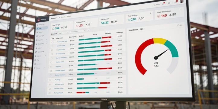
A construction job-cost model is the financial control system that connects your original estimate to real-world performance, giving you the data to protect margins before a project goes sideways.
Key Takeaways
- Over 85% of large construction projects run over budget or schedule, according to McKinsey Global Institute (2017), making granular cost tracking a survival skill, not a luxury.
- A job-cost model tracks direct costs (labor, materials, equipment, subcontractors) and indirect costs at the individual project level, unlike process costing which averages costs across production runs.
- Cost code structures tied to a Work Breakdown Structure (WBS) let you isolate variance at the phase, trade, or cost-type level — the difference between knowing you’re over budget and knowing exactly why.
- Earned Value Management (EVM) formulas — specifically Cost Performance Index (CPI) and Estimate at Completion (EAC) — give you a statistically grounded forecast of final cost from day one of construction.
- Labor burden rates in construction typically run 25%–40% above base wages when you include payroll taxes, workers’ compensation, benefits, and union fringes; omitting them is the single most common cause of labor cost overruns.
- ASC 606 percentage-of-completion revenue recognition requires job-cost data as its primary input, meaning your cost model directly drives your financial statements.
- A well-structured job-cost model across a portfolio of projects feeds a financial modeling framework that supports both project-level and company-level decision-making.
What Job-Cost Modeling Means in Construction Finance
Job-cost modeling is the practice of building a financial model for each individual construction project that tracks budgeted versus actual costs at a granular level, then uses that data to forecast final outcomes. It differs fundamentally from process costing (used in manufacturing, where identical units are produced repeatedly) because every construction project is unique: different site conditions, different subcontractor mixes, different risk profiles.
The Financial Accounting Standards Board defines job-order costing as the method appropriate when products or services are distinct and customer-specific. Construction fits that definition precisely. A commercial office fit-out in Chicago has nothing in common with a highway interchange in Texas, even if both are managed by the same contractor.
The practical implication: you cannot manage construction profitability with a single company-wide P&L. You need a model at the job level that rolls up to the company level, not the other way around.
Job costing assigns costs to unique projects; process costing averages across identical production runs — only job costing fits construction.
The Financial Architecture: Core Components of a Job-Cost Model
Every construction job-cost model contains four direct cost categories and a structured approach to indirect costs. Direct costs are those you can trace unambiguously to a specific project. Indirect costs require allocation.
Direct cost categories:
- Labor: Field wages multiplied by the labor burden rate (see Section 4 for burden calculation). Never use bare wages alone.
- Materials: Purchased materials consumed on the project, tracked by purchase order and delivery receipt.
- Equipment: Owned equipment charged at an internal rental rate; rented equipment at invoice cost.
- Subcontractors: Subcontract commitments, approved change orders, and amounts invoiced to date.
Indirect costs include project management salaries, site supervision, temporary facilities, insurance, bonding, and a share of company overhead. These require an allocation methodology — covered in Section 4.
Contingency is a separate line item, not a plug. Industry practice for commercial construction typically sets contingency at 5%–10% of direct costs during design development, stepping down to 2%–5% at construction documents, according to the Association for the Advancement of Cost Engineering International (AACE International).
Direct costs — labor, materials, equipment, and subcontractors — form the core of every construction job-cost model, with contingency held as a separate controlled reserve.
Cost Code Structures and WBS Integration
A cost code structure is the numbering system that organizes every dollar spent on a project into a consistent hierarchy. Without it, you can’t compare performance across projects or identify systemic estimating errors.
The most widely used hierarchy in U.S. commercial construction follows the CSI MasterFormat (Construction Specifications Institute), which organizes work into 50 divisions. A typical three-level cost code looks like this:
- Level 1 (Division): 03 — Concrete
- Level 2 (Phase/Section): 03 30 — Cast-in-Place Concrete
- Level 3 (Cost Type): 03 30 L — Labor, 03 30 M — Materials, 03 30 E — Equipment
The Work Breakdown Structure (WBS) maps the physical scope of work (foundations, structural steel, MEP rough-in) to the cost code hierarchy. When your WBS and cost codes align, every field timesheet entry, every purchase order, and every subcontractor invoice lands in the right bucket automatically.
How granular should you go? A rule of thumb: go one level deeper than you think you need during estimating, then aggregate for reporting. A $50M commercial project might carry 400–600 active cost codes. A $5M residential subdivision might need 80–120. The goal is actionable granularity — enough detail to isolate a problem, not so much that field supervisors spend more time coding than building.
A three-level cost code structure (Division, Section, Cost Type) maps every dollar to a specific scope of work, enabling precise variance analysis.
Direct vs. Indirect Costs: Allocation Methodologies That Preserve Accuracy
Direct costs are straightforward to assign. Indirect costs are where models break down. Two primary allocation methods apply in construction.
Traditional burden rate method: You calculate a single overhead rate as a percentage of direct labor cost (or direct cost total), then apply it uniformly across all projects. Simple to administer, but it penalizes labor-intensive projects and subsidizes equipment-heavy ones.
Activity-Based Costing (ABC): ABC (a method that assigns overhead costs to specific activities, then to projects based on how much of each activity they consume) produces more accurate allocations. A project requiring extensive project management attention absorbs more PM overhead than a straightforward repetitive project, even if both have similar direct labor costs. ABC is more complex to implement but significantly more accurate for mixed-portfolio contractors.
Labor burden calculation — worked example:
Assume a carpenter earns $35.00/hour base wage. The employer’s share of FICA taxes alone is 7.65% of wages (IRS), adding $2.68 per hour before any other burden components are counted. Here’s the full math:
| Burden Component | Rate | $/Hour |
|---|---|---|
| Base wage | — | $35.00 |
| FICA (Social Security + Medicare) | 7.65% | $2.68 |
| Federal/State Unemployment | 2.50% | $0.88 |
| Workers’ Compensation Insurance | 8.00% | $2.80 |
| General Liability (allocated) | 2.00% | $0.70 |
| Health & Dental Benefits | — | $4.50 |
| Retirement / 401(k) match | 3.00% | $1.05 |
| Total Burdened Rate | ~35.3% | $47.61 |
Using $35.00 instead of $47.61 in your estimate means you’re underpricing labor by 36%. On a project with 10,000 labor hours, that’s a $126,100 shortfall before you break ground.
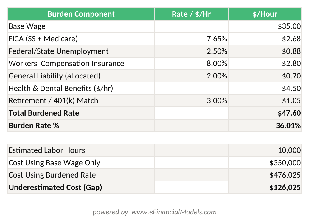
Labor burden adds 36% to base wages — on 10,000 hours, the difference between $35.00 and $47.61 is $126,100 in underestimated project cost.
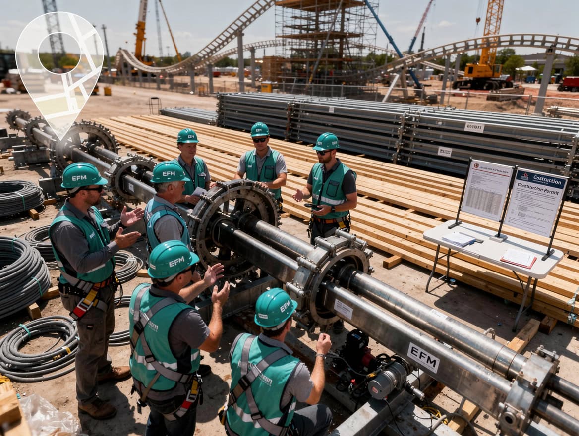
A 36% labor burden rate on a $35/hour carpenter adds $12.61/hour — on 10,000 hours, that’s $126,100 in underestimated cost if burden is ignored.
Building the Model: From Estimate to Baseline Budget
The baseline budget is the financial contract between the estimating team and the project team. It converts the bid estimate into a cost-code-level spending plan with time-phased cash flows.
The build sequence:
- Import the estimate into the job-cost model, mapped to cost codes. Every line item in the estimate gets a code.
- Adjust for scope changes between bid and contract award (value engineering, owner-directed changes).
- Phase the budget across the project schedule. A concrete pour in month 3 should show its cost in month 3, not spread evenly across 18 months.
- Set the contingency reserve as a separate, controlled line item — not embedded in individual cost codes.
- Lock the baseline. All subsequent changes go through a formal change management process that updates the budget and the contract value simultaneously.
The baseline budget becomes the denominator in every variance calculation you run for the life of the project. Protect it.
Real-Time Variance Analysis and Forecasting at Completion
Variance analysis compares what you planned to spend against what you actually spent, then projects where you’ll end up. Earned Value Management (EVM) provides the most rigorous framework for this in construction.
Core EVM terms (defined):
- Planned Value (PV): The budgeted cost of work scheduled to be complete by a given date.
- Earned Value (EV): The budgeted cost of work actually completed — what the completed work was worth in budget terms.
- Actual Cost (AC): What you actually spent to complete that work.
Key formulas:
- Cost Variance (CV) = EV – AC. Negative CV means you’re over budget for the work completed.
- Cost Performance Index (CPI) = EV / AC. A CPI of 0.92 means you’re spending $1.00 to deliver $0.92 of budgeted value.
- Estimate at Completion (EAC) = Budget at Completion (BAC) / CPI. This is your statistically derived forecast of final cost.
Worked example:
A $4,000,000 concrete package (BAC = $4,000,000) is 40% complete by schedule.
- PV = $4,000,000 × 40% = $1,600,000
- EV = $4,000,000 × 38% (actual percent complete) = $1,520,000
- AC = $1,680,000 (what you actually spent)
- CV = $1,520,000 – $1,680,000 = -$160,000 (over budget)
- CPI = $1,520,000 / $1,680,000 = 0.905
- EAC = $4,000,000 / 0.905 = $4,419,890
The model tells you: if current cost efficiency holds, this package will cost $419,890 more than budgeted. You have that information at 40% complete, not at project closeout.
The Project Management Institute’s PMBOK Guide notes that CPI established by the 20% completion point is statistically stable and rarely improves by more than 10% for the remainder of the project. That’s why early variance detection matters.
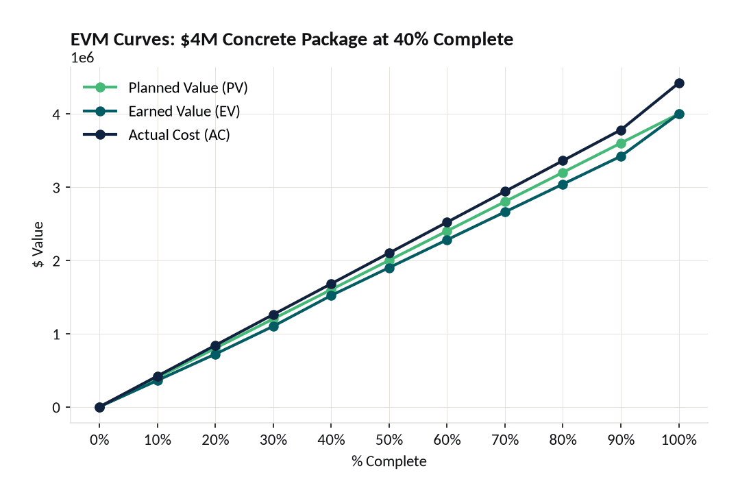
At 40% complete, Actual Cost ($1.68M) already exceeds Earned Value ($1.52M) by $160,000 — the CPI of 0.905 projects a final cost of $4.42M against a $4M budget.

When Actual Cost exceeds Earned Value, the CPI drops below 1.0 — and the EAC formula projects the final cost overrun automatically.
Revenue Recognition and Job-Cost Data Integration
ASC 606 (the revenue recognition standard issued by the Financial Accounting Standards Board, effective for public companies in 2018 and private companies in 2019) requires construction contractors to recognize revenue over time using a measure of progress. The most common measure: cost-to-cost percentage of completion.
The formula: Revenue recognized = (Costs incurred to date / Total estimated costs) × Contract value.
This means your job-cost model is not just a project management tool. It directly drives your income statement. An error in your cost-to-date figure or your estimate-to-complete produces a misstated revenue figure.
The integration architecture that supports accurate ASC 606 reporting typically flows as follows:
- Field: Daily timesheets, material receipts, and equipment logs captured in field management software.
- Accounting/ERP: Field data flows into the ERP (Enterprise Resource Planning system — the software that integrates accounting, procurement, and project data) via API or nightly batch.
- Job-Cost Model: The model pulls actuals from the ERP and compares them to the baseline budget, calculating percent complete and EAC.
- Financial Reporting: The percent complete and EAC feed the revenue recognition schedule, WIP (Work-in-Progress) report, and project-level P&L.
The WIP report — the document that reconciles contract value, billings, costs, and recognized revenue — is the output that auditors and lenders scrutinize most closely. Accurate job-cost data is its foundation. You can explore forecasting templates that support this data flow for multi-project portfolios.

Accurate ASC 606 revenue recognition depends on a clean data pipeline from field timesheets through the ERP to the job-cost model — any manual re-entry step introduces error.
Common Modeling Failures and How to Prevent Them
Most construction cost overruns trace back to a small set of modeling errors, not unpredictable site conditions.
1. Omitting or underestimating labor burden. As shown in Section 4, burden adds 25%–40% to base wages. Estimators who use bare labor rates consistently underbid labor-intensive scopes. Fix: build burden rates into your estimating database and update them annually.
2. Embedding contingency in cost codes. When estimators pad individual line items instead of carrying a separate contingency, you lose visibility into where risk actually sits. You also can’t release contingency systematically as risk burns off. Fix: zero-base each cost code and carry contingency as a controlled reserve.
3. Ignoring indirect cost allocation. Projects that consume disproportionate project management time, rework cycles, or executive attention are subsidized by simpler projects when you use a flat overhead rate. Fix: implement at minimum a two-rate system (field overhead vs. home office overhead) and consider ABC for complex portfolios.
4. Failing to update the estimate-to-complete. Many teams update actuals weekly but revise their estimate-to-complete only at monthly owner meetings. The EAC becomes stale within days. Fix: require project managers to update ETC (Estimate to Complete — the expected cost to finish remaining work) every two weeks at minimum.
5. Misaligning cost codes between estimate and accounting. When the estimating system uses different codes than the accounting system, costs land in wrong buckets and variance reports are meaningless. Fix: maintain a single master cost code library that both systems reference.
Most construction cost overruns trace to five modeling errors — all preventable with disciplined model design and update cadence.
Key Metrics: Measuring Financial Performance at the Job Level
A job-cost model generates the data for four metrics that construction CFOs should review on every active project.
| Metric | Formula | What It Tells You |
|---|---|---|
| Cost Performance Index (CPI) | EV / AC | Efficiency of cost spend; <1.0 = over budget |
| Cost Variance (CV) | EV – AC | Dollar over/under budget for work done |
| Estimate at Completion (EAC) | BAC / CPI | Projected final cost at current efficiency |
| Profit Fade | Bid margin – Current margin | Erosion of expected profit over project life |
Profit fade analysis (the tracking of how a project’s expected profit margin shrinks from bid to completion) is particularly valuable for identifying systemic estimating problems. If commercial projects consistently fade 3–5 margin points between award and 50% complete, your estimating assumptions are structurally wrong — not your field execution.
For multi-project portfolios, KPI tracking templates let you aggregate these metrics across jobs and identify which project types, project managers, or geographies consistently outperform or underperform.
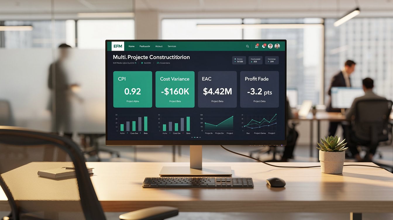
Portfolio-level KPI monitoring surfaces which project types, managers, or geographies consistently underperform — enabling systemic corrections rather than project-by-project firefighting.
Implementing Job-Cost Models Across Multiple Projects
Scaling job-cost modeling from one project to a portfolio requires standardization. Every project must use the same cost code structure, the same burden rates, and the same ETC update cadence — otherwise roll-up reporting is meaningless.
A practical implementation sequence:
- Standardize the cost code library across all projects. Publish it as a controlled document with version control.
- Build a model template with pre-loaded formulas for CPI, EAC, and percent complete. Project managers populate inputs; the model calculates outputs.
- Automate the actuals feed from your ERP. Manual data entry into job-cost models is the primary source of errors and delays.
- Establish a reporting cadence: weekly cost flash (actuals vs. budget by major cost code), monthly full variance report with updated EAC, quarterly profit fade review.
- Use performance tracking tools to monitor trends across the portfolio — which project types generate the most cost variance, which subcontractor categories consistently run over.
The construction financial managers who get this right treat the job-cost model as a living document, not a post-mortem. They update it continuously, challenge the ETC aggressively, and use it to make decisions — not to explain what already happened.
Frequently Asked Questions
What is the difference between job costing and process costing in construction?
Job costing assigns costs to individual, unique projects. Process costing averages costs across identical or near-identical units of production, which is appropriate for manufacturing but not construction. Every construction project has unique site conditions, contract terms, subcontractor mixes, and risk profiles. A highway contractor building 10 miles of identical pavement could theoretically use process costing for the paving operation, but the project as a whole — with its mobilization, drainage, structures, and traffic control — requires job costing. The Financial Accounting Standards Board’s guidance on revenue recognition under ASC 606 reinforces this: construction contracts are treated as distinct performance obligations, requiring project-level cost tracking to measure progress accurately.
How do I calculate the labor burden rate for my construction company?
Start with your base wage, then add every employer-paid cost associated with that employee. The standard components are: FICA taxes (7.65% of wages), federal and state unemployment taxes (typically 2%–3%), workers’ compensation insurance (varies by trade, from roughly 3% for clerical to 25%+ for ironworkers), general liability insurance (allocated portion), health and dental benefits (typically $3–$6/hour), retirement contributions, and any union fringe benefits. Sum all additions and divide by base wages to get your burden percentage. For a carpenter earning $35/hour with $12.61/hour in burden costs, the burden rate is 36% and the burdened rate is $47.61/hour. Update this calculation annually as insurance rates and benefit costs change.
What contingency percentage should I carry in a construction job-cost model?
Contingency should reflect the uncertainty remaining in the project scope and design at the time of estimating. AACE International’s recommended practice suggests 10%–20% of direct costs at the conceptual/schematic design phase, 5%–10% at design development, and 2%–5% at construction documents for commercial projects. Infrastructure projects with complex subsurface conditions or regulatory risk often carry higher contingency. The key discipline is carrying contingency as a separate, controlled line item — not embedded in individual cost codes — so you can release it systematically as risk is resolved and maintain visibility into how much buffer remains.
How does job-cost data feed ASC 606 revenue recognition?
ASC 606 requires contractors to recognize revenue over time when the customer controls the asset as it’s created. The cost-to-cost method measures progress as: costs incurred to date divided by total estimated costs, multiplied by the contract value. Your job-cost model provides both inputs: costs incurred to date (from actuals) and total estimated costs (from your current EAC). A $10M contract that is 42% complete by cost ($4.2M incurred out of $10M estimated total cost) recognizes $4.2M in revenue. If your EAC increases because costs are running over, the percent complete changes, which changes recognized revenue — sometimes creating a revenue reversal. Accurate job-cost data is therefore not just a project management tool; it’s an accounting input that affects your income statement and balance sheet.
What is profit fade and how do I detect it early?
Profit fade is the erosion of a project’s expected profit margin between bid and completion. A project bid at a 12% gross margin that closes at 7% has faded 5 margin points. Early detection requires comparing the current projected margin (contract value minus EAC, divided by contract value) to the bid margin at regular intervals — ideally monthly. A project fading more than 2 margin points by the 25% completion mark is a serious warning sign. Common causes include labor productivity assumptions that don’t hold in the field, subcontractor buyout savings that were assumed but not achieved, and scope growth that isn’t captured in approved change orders. The job-cost model surfaces these issues if you update the ETC honestly and frequently.
How granular should my cost code structure be?
The right level of granularity depends on project size and complexity. A practical benchmark: for projects under $5M, 80–150 cost codes typically provide sufficient visibility. For projects between $5M and $50M, 200–500 codes are common. For projects above $50M, 500+ codes may be warranted, particularly for complex MEP or civil work. The test is whether a project manager can identify the source of a variance within 15 minutes of reviewing the cost report. If the codes are too broad, variances are hidden. If they’re too granular, the administrative burden overwhelms the field team and data quality suffers. Align your cost code depth with your estimating detail — you can only track what you estimated.
What ERP or software systems support construction job costing?
The article intentionally avoids software vendor comparisons, but the integration architecture matters more than the specific tools. The critical requirement is a single master cost code library that your estimating system, field management software, and accounting/ERP system all reference. When these systems use different code structures, costs must be manually re-coded — introducing errors and delays. The data flow should be: field timesheets and material receipts captured daily in the field, flowing automatically into the accounting system, which feeds the job-cost model with actuals. Manual re-entry at any step in that chain is a control weakness. Prioritize integration capability over feature richness when evaluating systems.
Conclusion
Job-cost modeling is the financial infrastructure that separates contractors who know their margins from those who discover them at project closeout. The model connects your estimate to your actuals, your actuals to your forecast, and your forecast to your financial statements. Get the cost codes right, calculate burden rates accurately, update your ETC honestly, and apply EVM discipline from day one.
I recommend downloading the EFM Construction Financial Model to implement granular cost tracking, variance analysis, and EAC forecasting across your project portfolio — with pre-built cost code structures, burden rate calculators, and ASC 606 revenue recognition schedules ready to populate with your project data.