0 ITEMS

Excel Two Formulas in One Cell: Financial Modeling Guide
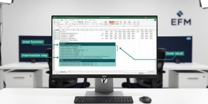
You can put two formulas in one Excel cell in three ways: nest one function inside another, join their outputs with the ampersand (&) operator, or link them with logical and mathematical operators. Which method fits depends on whether you need a multi-step calculation, a dynamic text label, or a conditional flag. Current versions of Excel let a single cell hold up to 8,192 characters and 64 levels of nested functions, so the real limit is rarely Excel itself — it is whether anyone can audit the result six months later. This guide walks through all three methods with worked financial modeling examples, Excel’s hard limits, debugging techniques, and the cases where helper columns beat a single combined formula.
Key Takeaways
- Excel supports up to 64 levels of nested functions and up to 8,192 characters per formula cell—knowing these limits prevents model-breaking errors before they happen.
- 88% of real-world spreadsheets contain errors according to EuSpRIG field audits, making disciplined formula construction a direct business risk control.
- Nested INDEX-MATCH with IFERROR is the industry-standard lookup pattern for financial statement models—it replaces fragile VLOOKUP chains with a single, auditable formula.
- The LAMBDA function (Excel 365 and Excel 2021+) lets you define reusable formula components, reducing formula duplication across large models.
- Helper columns are not a weakness—breaking a 200-character nested formula into 3 labeled steps often reduces audit time by more than combining everything into one cell saves.
- Named ranges transform unreadable nested formulas like
=IF(B7>C12,NPV(D2,E5:E14),0)into self-documenting expressions like=IF(Revenue>Threshold,NPV(DiscountRate,CashFlows),0).
Why Financial Modelers Combine Excel Formulas
Combining formulas in a single cell reduces the number of intermediate columns a model needs, keeps calculation logic in one auditable location, and enables dynamic outputs that update automatically when inputs change. The trade-off is real: a 150-character nested formula that took 20 minutes to write can take 2 hours to debug six months later.
Financial models live or die by their auditability. A DCF model (Discounted Cash Flow model: a valuation method that estimates the present value of future cash flows) with 40 tabs and hundreds of nested formulas is a liability if no one on the team can trace an error back to its source. The goal is not to minimize cell count—it is to maximize clarity per calculation.
According to a European Spreadsheet Risks Interest Group (EuSpRIG) review of field audits, 88% of real-world spreadsheets contained errors (EuSpRIG, 2013). A separate KPMG survey of 22 operational spreadsheets found that 91% contained significant errors, and 59% had serious calculation or control issues (KPMG, reported via EuSpRIG, 1998). These figures are not abstract—they represent valuation errors, misreported budgets, and flawed investment decisions.
Proper formula construction, including knowing when to combine and when to split, is one of the most direct ways to reduce that error rate.
The Three Core Methods of Combining Formulas in Excel
You can combine formulas in Excel using three distinct approaches: function nesting, text concatenation with the ampersand operator, and logical or mathematical operators that link formula outputs. Each method suits different financial modeling scenarios, and most complex models use all three.
Method 1: Function Nesting for Multi-Step Calculations
Function nesting means placing one function inside another so that the inner function’s result becomes an input (argument) to the outer function. Excel evaluates nested functions from the innermost outward.
A common financial modeling pattern nests IFERROR around INDEX-MATCH to handle missing data in lookup tables without returning ugly error codes to a board report:
=IFERROR(INDEX(RateTable,MATCH(B5,CompanyList,0),3),"Not Found")
Here, MATCH finds the row position of the company name in B5 within CompanyList. INDEX then retrieves the value from column 3 of RateTable at that row. IFERROR wraps the entire expression and returns “Not Found” if the lookup fails—rather than a #N/A error that breaks downstream calculations.
Current versions of Excel allow up to 64 levels of nested functions in a single formula, the ceiling Microsoft publishes in Excel specifications and limits, and Microsoft’s IF function documentation shows how to chain multiple IF tests within that budget. In practice, any formula requiring more than 5 or 6 levels of nesting is a strong signal to refactor into helper columns or a lookup table.
Method 2: Text Concatenation with the Ampersand Operator
The ampersand (&) operator joins text strings and formula results into a single cell output. Financial modelers use this constantly for dynamic report labels, scenario headers, and dashboard annotations that update automatically when assumptions change.
Example: a variance analysis dashboard that labels each row with the period and metric name:
="FY"&TEXT(B2,"YYYY")&" EBITDA Variance: "&TEXT(C5-D5,"$#,##0")
If B2 contains 2024, C5 contains actual EBITDA of $4,200,000, and D5 contains budgeted EBITDA of $3,800,000, this formula returns: FY2024 EBITDA Variance: $400,000.
The TEXT function (a formatting function that converts a number to a string with a specified format) is essential here—without it, the ampersand concatenates raw numbers without currency formatting. The TEXT function supports over 300 number format codes, catalogued in Microsoft’s TEXT function documentation, giving modelers precise control over how financial figures appear in dynamic labels.
Method 3: Logical and Mathematical Operators for Conditional Calculations
Logical operators (=, >, <, >=, <=, <>) and mathematical operators (+, -, *, /) connect formula components to produce conditional or compound results. In financial models, these appear most often in sensitivity analysis, covenant testing, and budget variance flags.
Example: a debt covenant test that flags a breach:
=IF(AND(DebtServiceCoverage<1.25, TotalDebt/EBITDA>4.0),"COVENANT BREACH","Compliant")
This formula uses AND (a logical function that returns TRUE only when all conditions are true) to test two conditions simultaneously. If both the DSCR (Debt Service Coverage Ratio: net operating income divided by total debt service) falls below 1.25 and leverage exceeds 4.0x, the cell flags a breach.
Excel’s Technical Limits: Characters, Nesting Depth, and Arguments
Every financial modeler needs to know Excel’s hard limits before building complex nested formulas, because hitting them mid-project causes formula truncation errors that are difficult to diagnose.
The now-retired Excel 2003 limited formulas to 1,024 characters per cell, whereas current versions of Excel support up to 8,192 characters in a single formula, a limit Microsoft publishes in Excel specifications and limits. That is an 8x increase, but a formula approaching 8,000 characters is almost certainly a maintainability problem regardless of whether it technically works.
Excel also supports a maximum of 255 arguments in a single function call — another figure from Microsoft’s Excel specifications and limits — allowing users to combine hundreds of references and expressions in one cell. The 255-argument limit matters most for SUM, IF arrays, and CHOOSE functions used in scenario switching. Additionally, a single Excel workbook can contain up to 1,024 open windows at one time according to Microsoft’s Excel specifications and limits, a reminder of just how expansive the platform’s architecture is relative to the formula-level constraints modelers typically encounter.
| Limit | Excel 2003 | Excel 2007+ (Current) |
|---|---|---|
| Characters per formula | 1,024 | 8,192 |
| Nested function levels | 7 | 64 |
| Arguments per function | 30 | 255 |
| Unique cell styles | 4,000 | 64,000 |
When a model approaches these limits, the right response is refactoring: move intermediate calculations to named ranges or helper columns, not cramming more characters into one cell.
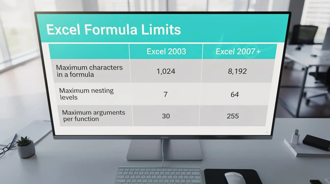
Excel’s 8x increase in formula character limit from 2003 to current versions expanded modeling capability—but formulas near the 8,192-character ceiling are almost always a maintainability problem.
Worked Example: Combining NPV, IF, and Conditional Logic
This example shows how to combine NPV (Net Present Value: the sum of discounted future cash flows minus the initial investment) with an IF statement to build an investment decision rule in a single cell.
Inputs:
- Discount rate (cell B2): 10%
- Cash flows years 1-5 (cells C2:G2): $500,000 / $600,000 / $700,000 / $800,000 / $900,000
- Initial investment (cell B3): $2,500,000
- Hurdle rate NPV threshold (cell B4): $0
Formula:
=IF(NPV(B2,C2:G2)-B3>B4,"INVEST: NPV = "&TEXT(NPV(B2,C2:G2)-B3,"$#,##0"),"REJECT: NPV = "&TEXT(NPV(B2,C2:G2)-B3,"$#,##0"))
Here’s the math:
NPV at 10% of the five cash flows:
- PV Year 1: $500,000 / 1.10 = $454,545
- PV Year 2: $600,000 / 1.21 = $495,868
- PV Year 3: $700,000 / 1.331 = $525,920
- PV Year 4: $800,000 / 1.4641 = $546,411
- PV Year 5: $900,000 / 1.61051 = $558,829
- Sum of PVs: $2,581,574
- Less initial investment: $2,581,574 – $2,500,000 = $81,574
Since $81,574 > $0, the formula returns: INVEST: NPV = $81,574.
This single cell delivers both the decision and the supporting figure—useful for executive summary dashboards where space is limited.

Combined IF-NPV formula: inputs in rows 2-3, cash flows in C2:G2, formula in B8 returns ‘INVEST: $81,574’ when NPV exceeds the hurdle threshold.
Worked Example: Nested INDEX-MATCH with IFERROR
INDEX-MATCH is the preferred lookup method in professional financial models because, unlike VLOOKUP, it can look left, handles column insertions without breaking, and performs faster on large datasets.
Scenario: a financial statement model that pulls the applicable tax rate for each entity from a reference table, returning a default rate if the entity is not listed.
=IFERROR(INDEX(TaxRateTable,MATCH(EntityName,EntityList,0),2),DefaultTaxRate)
- MATCH searches EntityList for the value in EntityName and returns its row number.
- INDEX retrieves the value from column 2 of TaxRateTable at that row number.
- IFERROR catches any #N/A or #REF! errors and substitutes DefaultTaxRate (a named range set to 21%).
Using named ranges (labels assigned to cell ranges that replace cryptic addresses like $B$2:$B$50 with readable names like EntityList) makes this formula self-documenting. Any analyst opening the model can read the formula logic without tracing cell references.

Named ranges like EntityList and TaxRateTable make the INDEX-MATCH lookup self-documenting—any analyst can read the formula logic without tracing cell addresses.
Debugging Complex Nested Formulas
Debugging nested formulas requires a systematic approach, not trial and error. Excel provides three tools that financial modelers should use in sequence.
Evaluate Formula (Formulas tab > Formula Auditing > Evaluate Formula): This tool steps through each component of a nested formula one evaluation at a time, showing the intermediate result at each stage. It is the single most useful debugging tool for formulas with 3+ nesting levels.
F9 partial evaluation: Select any sub-expression within a formula in the formula bar and press F9 to calculate just that portion. This isolates which component is returning an unexpected value. Press Escape (not Enter) to exit without committing the change.
Error trapping with IFERROR and ISERROR: Wrap suspect sub-expressions in IFERROR during development to identify which component fails. Once the error source is identified, fix the root cause rather than permanently masking it with IFERROR.
Common nested formula errors in financial models:
- Mismatched parentheses: Excel highlights unmatched parentheses in red. Count opening and closing parentheses before finalizing any formula with 3+ nesting levels.
- Mixed reference types: Using relative references (A1) inside a formula that gets copied across rows or columns shifts the reference unintentionally. Use absolute references ($A$1) for fixed inputs like discount rates and tax rates.
- Operator precedence errors: Excel follows standard mathematical order of operations (exponents first, then multiplication/division, then addition/subtraction).
=2+3*4returns 14, not 20. Use parentheses to enforce intended calculation order. - Volatile function overuse: Functions like NOW(), TODAY(), RAND(), and OFFSET() recalculate every time any cell in the workbook changes. Embedding them inside complex nested formulas in large models causes significant performance degradation.
- Array formula entry errors: Array formulas (formulas that perform calculations on multiple values simultaneously, entered with Ctrl+Shift+Enter in older Excel versions) must be entered correctly or they return a single value instead of an array result.
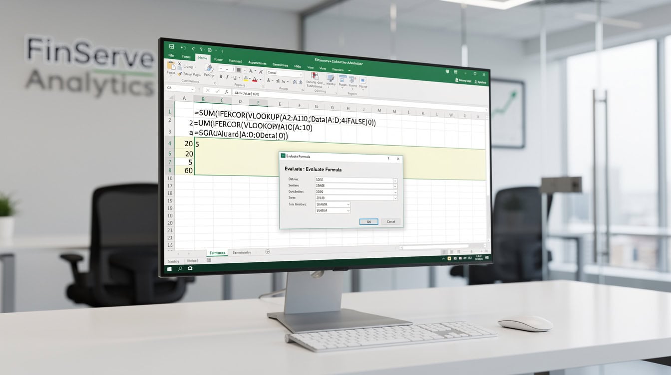
The Evaluate Formula tool steps through each nesting level sequentially—the most reliable debugging method for formulas with 3 or more nested functions.
When NOT to Combine Formulas
Combining formulas is not always the right choice. Knowing when to split calculations across helper columns is as important as knowing how to nest them.
Split formulas into helper columns when:
- The combined formula exceeds 100 characters and will be reviewed by external auditors.
- The formula contains more than 3 nesting levels and intermediate values have standalone analytical meaning (for example, gross margin before tax is worth showing separately from net margin).
- The model follows the FAST Standard (a financial modeling best practice framework that mandates one formula per row, consistent structure, and full audit traceability) or similar audit-focused conventions.
- The formula will be maintained by analysts who did not build it.
Split formulas into helper columns when the combined version creates a “black box” calculation: a formula whose output cannot be verified by inspection without running the Evaluate Formula tool. Black box formulas fail audit reviews and create restatement risk in regulated financial reporting.
| Scenario | Combine in One Cell | Use Helper Columns |
|---|---|---|
| Executive dashboard label | Yes | No |
| DCF terminal value calculation | No | Yes |
| Covenant compliance flag | Yes | No |
| Multi-step IRR sensitivity | No | Yes |
| Dynamic report header | Yes | No |
| Three-statement model link | No | Yes |

Helper columns are not a weakness—a 3-step labeled calculation that any analyst can follow in 60 seconds outperforms a single-cell formula that requires diagnostic tools to decode.
Best Practices for Formula Construction in Financial Models
Professional financial models follow consistent conventions that make complex nested formulas readable, auditable, and maintainable.
Use named ranges for all key inputs. A formula reading =IF(Revenue>Threshold,NPV(DiscountRate,CashFlows),0) communicates intent immediately. The equivalent =IF(B7>C12,NPV(D2,E5:E14),0) requires the reader to navigate to four separate cells before understanding the logic. You can define named ranges via Formulas > Name Manager.
Document formula logic in adjacent cells. A short note in column A explaining what a complex formula in column B calculates takes 30 seconds to write and saves hours during model reviews.
Use LAMBDA for reusable formula components (Excel 365 and Excel 2021+). LAMBDA (a function that lets you define custom, reusable functions without VBA) eliminates the need to copy identical nested formulas across multiple cells. Define the logic once, name it, and call it by name anywhere in the workbook.
Test formulas with boundary values. Before finalizing any nested formula in a financial model, test it with zero inputs, negative values, and blank cells. These edge cases expose errors that normal test data misses.
For analysts building models from scratch, the Excel financial model templates available through EFM demonstrate these conventions applied to real DCF, LBO, and budget models. The Information Technology Industry Business Excel Model shows how professional modelers structure nested formulas across multi-tab workbooks.
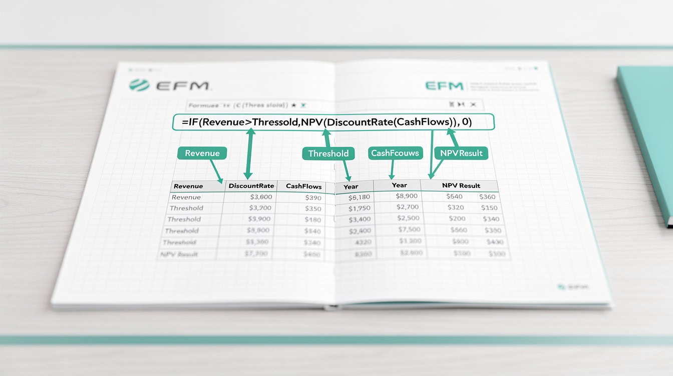
Named ranges transform cryptic cell addresses into readable formula logic—a 30-second investment that saves hours during model reviews and audits.
Frequently Asked Questions
How do you put two formulas in one Excel cell without errors?
The safest approach is to nest the secondary formula as an argument inside the primary formula, then wrap the entire expression in IFERROR to catch any runtime errors. For example, to combine a conditional check with a financial calculation: =IFERROR(IF(Revenue>0,NPV(DiscountRate,CashFlows),0),"Input Error"). Before finalizing, use the Evaluate Formula tool (Formulas tab > Formula Auditing) to step through each component and confirm intermediate results match expectations. Test with zero, negative, and blank inputs to expose edge cases. Formulas combining 3 or more functions should always be tested against at least 5 different input scenarios before deployment in a live model.
What is the difference between nesting functions and using the ampersand operator?
Nesting functions means placing one function inside another so the inner result feeds the outer calculation—for example, =IFERROR(INDEX(...),"N/A"). The ampersand (&) operator concatenates (joins) text strings and formula outputs into a single text value—for example, ="EBITDA: "&TEXT(C5,"$#,##0"). Nesting is used for multi-step numerical calculations. The ampersand is used for dynamic labels, report headers, and dashboard annotations. You can combine both in one cell: =IF(NPV(Rate,Flows)>0,"Positive NPV: "&TEXT(NPV(Rate,Flows),"$#,##0"),"Negative NPV"). This formula nests NPV inside IF and uses the ampersand to format the output as a readable string.
How many formulas can you nest in one Excel cell?
Current versions of Excel allow up to 64 levels of nested functions in a single formula, and up to 8,192 characters total per cell. In practice, formulas exceeding 5-6 nesting levels become difficult to audit and maintain. The FAST Standard and similar financial modeling frameworks recommend keeping formulas simple enough that a qualified analyst can verify the logic by reading the formula bar without running diagnostic tools. If you need more than 6 nesting levels, consider refactoring into helper columns with named ranges, or using LAMBDA (available in Excel 365 and Excel 2021+) to define reusable sub-formulas.
Why do my nested formulas return wrong results in financial models?
The most common causes are: incorrect operator precedence (Excel multiplies before it adds, so =2+3*4 returns 14 not 20—use parentheses to enforce order), mixed relative and absolute references that shift when formulas are copied, and volatile functions like OFFSET() or INDIRECT() that recalculate unexpectedly. In financial models specifically, a frequent error is referencing a cell that contains another formula rather than a hard-coded input, creating circular reference chains. Use F9 to evaluate sub-expressions in the formula bar and isolate which component returns the unexpected value. The Evaluate Formula tool steps through each calculation stage and shows the intermediate result.
When should I use helper columns instead of combining formulas?
Use helper columns when the combined formula exceeds roughly 100 characters, when intermediate values have standalone analytical meaning (gross margin before tax is worth showing separately), or when the model will be reviewed by external auditors who need to trace every calculation step. The FAST Standard, a widely adopted financial modeling best practice framework, explicitly recommends one calculation per row and consistent formula structure across columns. A 3-line helper column calculation that any analyst can follow in 60 seconds is more valuable than a single-cell formula that requires the Evaluate Formula tool to decode. For general Excel financial models, helper columns also make sensitivity analysis easier because each intermediate step can be independently stress-tested.
Does the LAMBDA function replace nested formulas in Excel 365?
LAMBDA does not replace nested formulas—it makes them reusable. LAMBDA (available in Excel 365 and Excel 2021+) lets you define a custom function with named parameters and assign it a name via the Name Manager. Once defined, you call it like any built-in function. For example, you could define a LAMBDA called AdjustedEBITDA that takes Revenue, COGS, and OpEx as parameters and returns Revenue-COGS-OpEx. Every cell in the model that needs adjusted EBITDA then calls =AdjustedEBITDA(B5,C5,D5) instead of repeating the same nested formula. This reduces formula duplication, makes updates a single-point change, and dramatically improves model auditability. LAMBDA is not available in Excel 2019 or earlier.
How do I combine NPV with conditional logic for investment screening?
The standard pattern nests Excel’s NPV function inside an IF statement: =IF(NPV(DiscountRate,CashFlows)-InitialInvestment>HurdleNPV,"INVEST","REJECT"). NPV (Net Present Value) calculates the present value of future cash flows discounted at the specified rate. Subtracting the initial investment gives the true NPV. The IF function then compares that NPV against a hurdle threshold. For a more informative output, combine with the ampersand: =IF(NPV(B2,C2:G2)-B3>0,"INVEST: "&TEXT(NPV(B2,C2:G2)-B3,"$#,##0"),"REJECT: "&TEXT(NPV(B2,C2:G2)-B3,"$#,##0")). Note that Excel’s NPV function assumes cash flows occur at end-of-period. For irregular timing, use XNPV instead, which accepts explicit date arguments. You can explore ready-built investment screening models in the EFM Excel template library.
Conclusion
Combining two formulas in one Excel cell is a core financial modeling skill, but the goal is always clarity and auditability, not formula brevity for its own sake. The 88% spreadsheet error rate documented by EuSpRIG is a direct consequence of formulas that prioritize compactness over transparency. Use nesting for multi-step calculations, the ampersand for dynamic labels, and logical operators for conditional outputs. Know Excel’s limits: 8,192 characters, 64 nesting levels, 255 arguments. And know when to stop: helper columns, named ranges, and LAMBDA functions often produce more maintainable models than a single 200-character nested expression.
I recommend downloading the EFM Excel financial model templates to see these formula construction techniques applied in professionally built DCF, LBO, and budget models—complete with named ranges, documented helper columns, and IFERROR error handling throughout.